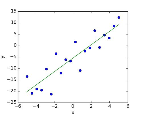
Fit a simple linear regression using ‘statsmodels’, compute corresponding p-values.
Script output:
  OLS Regression Results
==============================================================================
Dep. Variable:                      y   R-squared:                       0.804
Model:                            OLS   Adj. R-squared:                  0.794
Method:                 Least Squares   F-statistic:                     74.03
Date:                Wed, 26 Aug 2015   Prob (F-statistic):           8.56e-08
Time:                        10:15:04   Log-Likelihood:                -57.988
No. Observations:                  20   AIC:                             120.0
Df Residuals:                      18   BIC:                             122.0
Df Model:                           1
==============================================================================
                 coef    std err          t      P>|t|      [95.0% Conf. Int.]
------------------------------------------------------------------------------
Intercept     -5.5335      1.036     -5.342      0.000        -7.710    -3.357
x              2.9369      0.341      8.604      0.000         2.220     3.654
==============================================================================
Omnibus:                        0.100   Durbin-Watson:                   2.956
Prob(Omnibus):                  0.951   Jarque-Bera (JB):                0.322
Skew:                          -0.058   Prob(JB):                        0.851
Kurtosis:                       2.390   Cond. No.                         3.03
==============================================================================

ANOVA results
          df       sum_sq      mean_sq          F        PR(>F)
x          1  1588.873443  1588.873443  74.029383  8.560649e-08
Residual  18   386.329330    21.462741        NaN           NaN
Python source code: plot_regression.py
# Original author: Thomas Haslwanter

import numpy as np
import matplotlib.pyplot as plt
import pandas

# For statistics. Requires statsmodels 5.0 or more
from statsmodels.formula.api import ols
# Analysis of Variance (ANOVA) on linear models
from statsmodels.stats.anova import anova_lm

##############################################################################
# Generate and show the data
x = np.linspace(-5, 5, 20)

# To get reproducable values, provide a seed value
np.random.seed(1)

y = -5 + 3*x + 4 * np.random.normal(size=x.shape)

# Plot the data
plt.figure(figsize=(5, 4))
plt.plot(x, y, 'o')

##############################################################################
# Multilinear regression model, calculating fit, P-values, confidence
# intervals etc.

# Convert the data into a Pandas DataFrame to use the formulas framework
# in statsmodels
data = pandas.DataFrame({'x': x, 'y': y})

# Fit the model
model = ols("y ~ x", data).fit()

# Print the summary
print(model.summary())

# Peform analysis of variance on fitted linear model
anova_results = anova_lm(model)

print('\nANOVA results')
print(anova_results)

##############################################################################
# Plot the fitted model

# Retrieve the parameter estimates
offset, coef = model._results.params
plt.plot(x, x*coef + offset)
plt.xlabel('x')
plt.ylabel('y')

plt.show()
Total running time of the example: 0.14 seconds ( 0 minutes 0.14 seconds)
