1.1. Metrics to judge the sucess of a model

Pro & cons of various performance metrics.

The simple way to use a scoring metric during cross-validation is via the scoring parameter of sklearn.model_selection.cross_val_score().

1.1.1. Regression settings

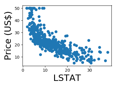
1.1.1.1. The Boston housing data

from sklearn import datasets
boston = datasets.load_boston()

# Shuffle the data
from sklearn.utils import shuffle
data, target = shuffle(boston.data, boston.target, random_state=0)

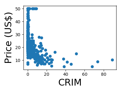
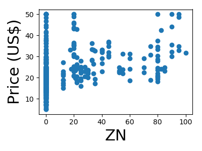
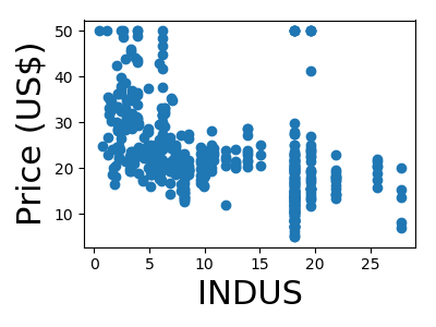
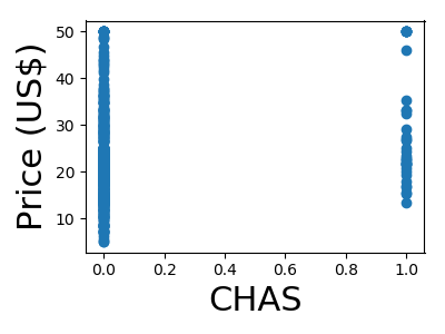
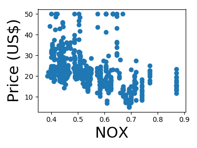
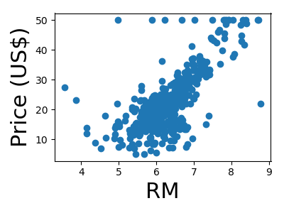
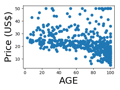
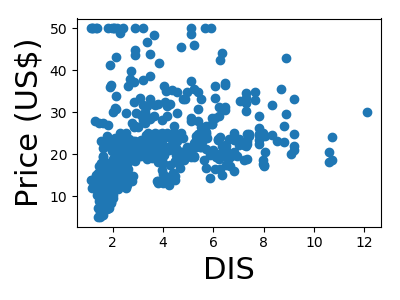
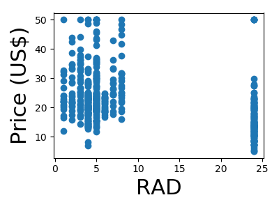
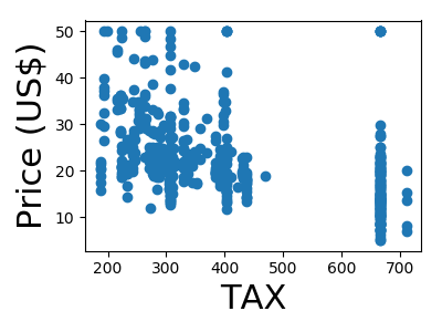
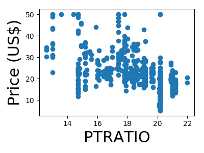
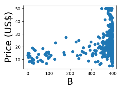
A quick plot of how each feature is related to the target

from matplotlib import pyplot as plt

for feature, name in zip(data.T, boston.feature_names):
    plt.figure(figsize=(4, 3))
    plt.scatter(feature, target)
    plt.xlabel(name, size=22)
    plt.ylabel('Price (US$)', size=22)
    plt.tight_layout()

• 
• 
• 
• 
• 
• 
• 
• 
• 
• 
• 
• 
• 

We will be using a random forest regressor to predict the price

from sklearn.ensemble import RandomForestRegressor
regressor = RandomForestRegressor()

1.1.1.2. Explained variance vs Mean Square Error

The default score is explained variance

from sklearn.model_selection import cross_val_score
print(cross_val_score(regressor, data, target))

Out:

[ 0.80185876  0.83501125  0.83122505]

Explained variance is convienent because it has a natural scaling: 1 is perfect prediction, and 0 is around chance

Now let us see which houses are easier to predict:

Not along the Charles river (feature 3)

print(cross_val_score(regressor, data[data[:, 3] == 0],
                      target[data[:, 3] == 0]))

Out:

[ 0.78068719  0.87449332  0.82714336]

Along the Charles river

print(cross_val_score(regressor, data[data[:, 3] == 1],
                      target[data[:, 3] == 1]))

Out:

[ 0.47939268 -0.23091137  0.83871587]

So the houses along the Charles are harder to predict?

It is not so easy to conclude this from the explained variance: in two different sets of observations, the variance of the target differs, and the explained variance is a relative measure

MSE: We can use the mean squared error (here negated)

Not along the Charles river

print(cross_val_score(regressor, data[data[:, 3] == 0],
                      target[data[:, 3] == 0],
                      scoring='neg_mean_squared_error'))

Out:

[-14.84768471  -8.53250191 -16.77990573]

Along the Charles river

print(cross_val_score(regressor, data[data[:, 3] == 1],
                      target[data[:, 3] == 1],
                      scoring='neg_mean_squared_error'))

Out:

[-80.363225   -62.05679167 -28.57741818]

So the error is larger along the Charles river

1.1.1.3. Mean Squared Error versus Mean Absolute Error

What if we want to report an error in dollars, meaningful for an application?

The Mean Absolute Error is useful for this goal

print(cross_val_score(regressor, data, target,
                      scoring='neg_mean_absolute_error'))

Out:

[-2.51940828 -2.26195266 -2.52642857]

1.1.1.4. Summary

• explained variance: scaled with regards to chance: 1 = perfect, 0 = around chance, but it shouldn’t used to compare predictions across datasets
• mean absolute error: enables comparison across datasets in the units of the target

1.1.2. Classification settings

1.1.2.1. The digits data

digits = datasets.load_digits()
# Let us try to detect sevens:
sevens = (digits.target == 7)

from sklearn.ensemble import RandomForestClassifier
classifier = RandomForestClassifier()

1.1.2.2. Accuracy and its shortcomings

The default metric is the accuracy: the averaged fraction of success. It takes values between 0 and 1, where 1 is perfect prediction

print(cross_val_score(classifier, digits.data, sevens))

Out:

[ 0.97333333  0.97662771  0.98160535]

However, a stupid classifier can each good prediction wit imbalanced classes

from sklearn.dummy import DummyClassifier
most_frequent = DummyClassifier(strategy='most_frequent')
print(cross_val_score(most_frequent, digits.data, sevens))

Out:

[ 0.9         0.89983306  0.90133779]

Balanced accuracy (available in scikit-learn 0.20) fixes this, but can have surprising behaviors, such as being negative, and can only be used for binary classification.

print(cross_val_score(classifier, digits.data, sevens,
                      scoring='balanced_accuracy'))

Out:

[ 0.85833333  0.93240569  0.93882268]

1.1.2.3. Precision, recall, and their shortcomings

We can measure separately false detection and misses

Precision: Precision counts the ratio of detections that are correct

print(cross_val_score(classifier, digits.data, sevens,
                      scoring='precision'))

Out:

[ 1.          1.          0.98039216]

Our classifier has a good precision: most of the sevens that it predicts are really sevens.

As predicting the most frequent never predicts sevens, precision is ill defined. Scikit-learn puts it to zero

print(cross_val_score(most_frequent, digits.data, sevens,
                      scoring='precision'))

Out:

[ 0.  0.  0.]

Recall: Recall counts the fraction of class 1 actually detected

print(cross_val_score(classifier, digits.data, sevens, scoring='recall'))

Out:

[ 0.73333333  0.8         0.84745763]

Our recall isn’t as good: we miss many sevens

But predicting the most frequent never predicts sevens:

print(cross_val_score(most_frequent, digits.data, sevens, scoring='recall'))

Out:

[ 0.  0.  0.]

Note: Measuring only the precision without the recall makes no sense, it is easy to maximize one at the cost of the other. Ideally, classifiers should be compared on a precision at a given recall

1.1.2.4. Area under the ROC curve

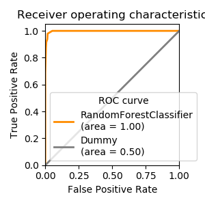
If the classifier provides a decision function that can be thresholded to control false positives versus false negatives, the ROC curve summarise the different tradeoffs that can be achieved by varying this threshold.

Its Area Under the Curve (AUC) is a useful metric where 1 is perfect prediction and .5 is chance, independently of class imbalance

print(cross_val_score(classifier, digits.data, sevens, scoring='roc_auc'))

Out:

[ 0.98606481  0.99795918  0.99927675]

print(cross_val_score(most_frequent, digits.data, sevens, scoring='roc_auc'))

Out:

[ 0.5  0.5  0.5]

1.1.2.4.1. Average precision

When the classifier exposes its unthresholded decision, another interesting metric is the average precision for all recall. Compared to ROC AUC it has a more linear behavior for very rare classes. Indeed, with very rare classes, small changes in the ROC AUC may mean large changes in terms of precision

print(cross_val_score(classifier, digits.data, sevens,
                      scoring='average_precision'))

Out:

[ 0.93169079  0.98168713  0.98500183]

Naive decisions are no longer at .5

print(cross_val_score(most_frequent, digits.data, sevens,
                      scoring='average_precision'))

Out:

[ 0.1         0.10016694  0.09866221]

1.1.2.5. Multiclass and multilabel settings

To simplify the discussion, we have reduced the problem to detecting sevens, but maybe it is more interesting to predict the digit: a 10-class classification problem

Accuracy The accuracy is naturally defined in such multiclass settings

print(cross_val_score(classifier, digits.data, digits.target))

Out:

[ 0.87873754  0.91318865  0.90100671]

The most frequent label is no longer a very interesting baseline

random_choice = DummyClassifier()
print(cross_val_score(random_choice, digits.data, digits.target))

Out:

[ 0.11295681  0.08013356  0.08892617]

Precision and recall need the notion of specific class to detect (called positive class) and are not that easily defined in these settings, hence ROC AUC cannot be easily computed.

These notions are however well defined in a multi-label problem. In such a problem, the goal is to assign one or more labels to each instance, as opposed to a multiclass. A multiclass problem can be turned into a multilabel one, though the prediction will then be slightly different

from sklearn.preprocessing import LabelBinarizer
digit_labels = LabelBinarizer().fit_transform(digits.target)
print(digit_labels[:15])

Out:

[[1 0 0 0 0 0 0 0 0 0]
 [0 1 0 0 0 0 0 0 0 0]
 [0 0 1 0 0 0 0 0 0 0]
 [0 0 0 1 0 0 0 0 0 0]
 [0 0 0 0 1 0 0 0 0 0]
 [0 0 0 0 0 1 0 0 0 0]
 [0 0 0 0 0 0 1 0 0 0]
 [0 0 0 0 0 0 0 1 0 0]
 [0 0 0 0 0 0 0 0 1 0]
 [0 0 0 0 0 0 0 0 0 1]
 [1 0 0 0 0 0 0 0 0 0]
 [0 1 0 0 0 0 0 0 0 0]
 [0 0 1 0 0 0 0 0 0 0]
 [0 0 0 1 0 0 0 0 0 0]
 [0 0 0 0 1 0 0 0 0 0]]

The ROC AUC can then be computed for each label, and the mean is reported

print(cross_val_score(classifier, digits.data, digit_labels,
                      scoring='roc_auc'))

Out:

[ 0.98369166  0.9886015   0.98884622]

as well as the average precision

print(cross_val_score(classifier, digits.data, digit_labels,
                      scoring='average_precision'))

Out:

[ 0.93498163  0.94880999  0.93500118]

Note that the confusion between classes may not well be captured in Such a measure, as in multiclass predictions are exclusive, and not in multilabel.

1.1.2.6. Summary

Class imbalance and the tradeoffs between accepting many misses or many false detections are the things to keep in mind in classification.

In single-class settings, ROC AUC and average precision give nice summaries to compare classifiers when the threshold can be varied. In multiclass settings, this is harder, unless we are willing to consider the problem as multiple single-class problems (one-vs-all).

---

Total running time of the script: ( 0 minutes 2.456 seconds)