1.2. Cross-validation: some gotchas

Cross-validation is the ubiquitous test of a machine learning model. Yet many things can go wrong.

1.2.1. Uncertainty of measured accuracy

1.2.1.1. Variations in cross_val_score: simple experiments

The first thing to have in mind is that the results of a cross-validation are noisy estimate of the real prediction accuracy

Let us create a simple artificial data

from sklearn import datasets, discriminant_analysis
import numpy as np
np.random.seed(0)
data, target = datasets.make_blobs(centers=[(0, 0), (0, 1)], n_samples=100)
classifier = discriminant_analysis.LinearDiscriminantAnalysis()

One cross-validation gives spread out measures

from sklearn.model_selection import cross_val_score
print(cross_val_score(classifier, data, target))

Out:

[ 0.64705882  0.67647059  0.84375   ]

What if we try different random shuffles of the data?

from sklearn import utils
for _ in range(10):
    data, target = utils.shuffle(data, target)
    print(cross_val_score(classifier, data, target))

Out:

[ 0.76470588  0.70588235  0.65625   ]
[ 0.70588235  0.67647059  0.75      ]
[ 0.73529412  0.64705882  0.71875   ]
[ 0.70588235  0.58823529  0.8125    ]
[ 0.67647059  0.73529412  0.71875   ]
[ 0.70588235  0.64705882  0.75      ]
[ 0.67647059  0.67647059  0.71875   ]
[ 0.70588235  0.61764706  0.8125    ]
[ 0.76470588  0.76470588  0.59375   ]
[ 0.76470588  0.61764706  0.625     ]

1.2.1.2. A simple probabilistic model

A sample probabilistic model gives the distribution of observed error: if the classification rate is p, the observed distribution of correct classifications on a set of size follows a binomial distribution

from scipy import stats
n = len(data)
distrib = stats.binom(n=n, p=.7)

We can plot it:

from matplotlib import pyplot as plt
plt.figure(figsize=(6, 3))
plt.plot(np.linspace(0, 1, n), distrib.pmf(np.arange(0, n)))

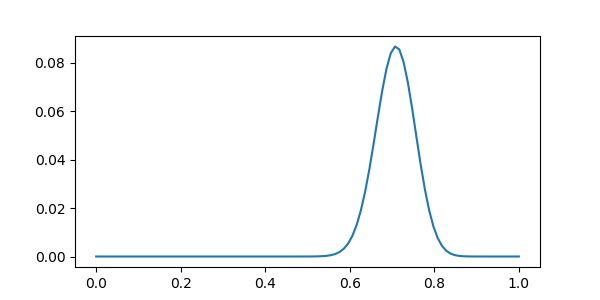
It is wide, because there are not that many samples to mesure the error upon: this is a small dataset.

We can look at the interval in which 95% of the observed accuracy lies for different sample sizes

for n in [100, 1000, 10000, 100000, 1000000]:
    distrib = stats.binom(n, .7)
    interval = (distrib.isf(.025) - distrib.isf(.975)) / n
    print("Size: {0: 8}  | interval: {1}%".format(n, 100 * interval))

Out:

Size:      100  | interval: 18.0%
Size:     1000  | interval: 5.7%
Size:    10000  | interval: 1.8%
Size:   100000  | interval: 0.568%
Size:  1000000  | interval: 0.1796%

At 100 000 samples, 5% of the observed classification accuracy still fall more than .5% away of the true rate.

Keep in mind that cross-val is a noisy measure

1.2.1.3. Empirical distribution of cross-validation scores

We can sample the distribution of scores using cross-validation iterators based on subsampling, such as sklearn.model_selection.ShuffleSplit, with many many splits

from sklearn import model_selection
cv = model_selection.ShuffleSplit(n_splits=200)
scores = cross_val_score(classifier, data, target, cv=cv)

import seaborn as sns
plt.figure(figsize=(6, 3))
sns.distplot(scores)
plt.xlim(0, 1)

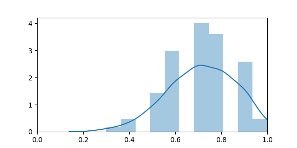
The empirical distribution is broader than the theoretical one. This can be explained by the fact that as we are retraining the model on each fold, it actually fluctuates due the sampling noise in the training data, while the model above only accounts for sampling noise in the test data.

The situation does get better with more data:

data, target = datasets.make_blobs(centers=[(0, 0), (0, 1)], n_samples=1000)

scores = cross_val_score(classifier, data, target, cv=cv)

plt.figure(figsize=(6, 3))
sns.distplot(scores)
plt.xlim(0, 1)
plt.title("Distribution with 1000 data points")

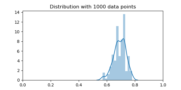
The distribution is still very broader

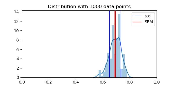
Testing the observed scores

Importantly, the standard error of the mean across folds is not a good measure of this error, as the different data folds are not independent. For instance, doing many random splits will can reduce the variance arbitrarily, but does not provide actually new data points

from scipy import stats

plt.figure(figsize=(6, 3))
sns.distplot(scores)
plt.axvline(np.mean(scores), color='k')
plt.axvline(np.mean(scores) + np.std(scores), color='b', label='std')
plt.axvline(np.mean(scores) - np.std(scores), color='b')
plt.axvline(np.mean(scores) + stats.sem(scores), color='r', label='SEM')
plt.axvline(np.mean(scores) - stats.sem(scores), color='r')
plt.legend(loc='best')
plt.xlim(0, 1)
plt.title("Distribution with 1000 data points")

1.2.1.4. Measuring baselines and chance

Because of class imbalances, or confounding effects, it is easy to get it wrong it terms of what constitutes chances. There are two approaches to measure peformances of baselines or chance:

DummyClassifier The dummy classifier: sklearn.dummy.DummyClassifier, with different strategies to provide simple baselines

from sklearn.dummy import DummyClassifier
dummy = DummyClassifier(strategy="stratified")
dummy_scores = cross_val_score(dummy, data, target)
print(dummy_scores)

Out:

[ 0.46407186  0.5         0.52409639]

Chance level To measure actual chance, the most robust approach is to use permutations: sklearn.model_selection.permutation_test_score(), which is used as cross_val_score

from sklearn.model_selection import permutation_test_score
score, permuted_scores, p_value = permutation_test_score(classifier,
                                                         data, target)
print("Classifier score: {0},\np value: {1}\nPermutation scores {2}"
        .format(score, p_value, permuted_scores))

Out:

Classifier score: 0.688021547267,
p value: 0.00990099009901
Permutation scores [ 0.50095592  0.51507227  0.52098814  0.48998389  0.4679797   0.50700406
  0.51100209  0.52801626  0.52193805  0.51599211  0.48692975  0.5420304
  0.48302792  0.49500998  0.51605824  0.49100594  0.48499988  0.51793401
  0.51800014  0.50495996  0.53599428  0.50098598  0.51700815  0.48302191
  0.51301614  0.53803237  0.51294399  0.50394392  0.46502176  0.48797586
  0.49000192  0.50402809  0.49799798  0.51706827  0.4680278   0.49699998
  0.52394007  0.50892793  0.52202222  0.49301998  0.4809778   0.51200611
  0.48095977  0.49797393  0.51700214  0.49796792  0.52795614  0.50200202
  0.47405791  0.49904408  0.51194599  0.49001395  0.50799004  0.49093981
  0.50598201  0.48697785  0.53200827  0.49102398  0.48497583  0.50303008
  0.51102013  0.46201573  0.5200202   0.50103408  0.52005026  0.481074
  0.48202992  0.52198014  0.53108241  0.50101604  0.50400404  0.53400428
  0.48401991  0.5320203   0.47397975  0.46098766  0.49798596  0.50091985
  0.4769437   0.49303802  0.51002814  0.4929779   0.50993796  0.51700214
  0.53998629  0.51301614  0.49906212  0.47192963  0.52991006  0.51099608
  0.48801193  0.48895582  0.48404396  0.50301806  0.50304211  0.5189741
  0.51494     0.48407402  0.49101796  0.50002405]

We can plot all the scores

plt.figure(figsize=(6, 3))
sns.distplot(dummy_scores, color="g", label="Dummy scores")
sns.distplot(permuted_scores, color="r", label="Permuted scores")
sns.distplot(scores, label="Cross validation scores")
plt.legend(loc='best')
plt.xlim(0, 1)

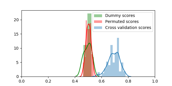
Permutation and performing many cross-validation splits are computationally expensive, but they give trust-worthy answers

1.2.2. Cross-validation with non iid data

Another common caveat for cross-validation are dependencies in the observations that can easily creep in between the train and the test sets. Let us explore these problems in two settings.

1.2.2.1. Stock market: time series

Download: Download and load the data:

import pandas as pd
import os
# Python 2 vs Python 3:
try:
    from urllib.request import urlretrieve
except ImportError:
    from urllib import urlretrieve

symbols = {'TOT': 'Total', 'XOM': 'Exxon', 'CVX': 'Chevron',
           'COP': 'ConocoPhillips', 'VLO': 'Valero Energy'}

quotes = pd.DataFrame()

for symbol, name in symbols.items():
    url = ('https://raw.githubusercontent.com/scikit-learn/examples-data/'
           'master/financial-data/{}.csv')
    filename = "{}.csv".format(symbol)
    if not os.path.exists(filename):
        urlretrieve(url.format(symbol), filename)
    this_quote = pd.read_csv(filename)
    quotes[name] = this_quote['open']

Prediction: Predict ‘Chevron’ from the others

from sklearn import linear_model, model_selection, ensemble
cv = model_selection.ShuffleSplit(random_state=0)
print(cross_val_score(linear_model.RidgeCV(),
                      quotes.drop(columns=['Chevron']),
                      quotes['Chevron'],
                      cv=cv).mean())

Out:

0.255791000942

Is this a robust prediction?

Does it cary over across quarters?

Stratification: To thest this we need to stratify cross-validation using a sklearn.model_selection.LeaveOneGroupOut

quarters = pd.to_datetime(this_quote['date']).dt.to_period('Q')
cv = model_selection.LeaveOneGroupOut()

print(cross_val_score(linear_model.RidgeCV(),
                      quotes.drop(columns=['Chevron']),
                      quotes['Chevron'],
                      cv=cv, groups=quarters).mean())

Out:

-55.0821056887

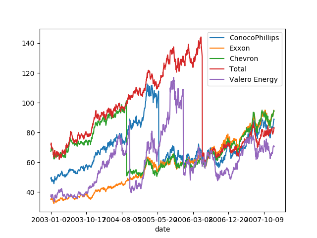
The problem that we are facing here is the auto-correlation in the data: these datasets are time-series.

quotes_with_dates = pd.concat((quotes, this_quote['date']),
                              axis=1).set_index('date')
quotes_with_dates.plot()

Testing for forecasting: If the goal is to do forecasting, than prediction should be done in the future, for instance using sklearn.model_selection.TimeSeriesSplit

Can we do forecasting: predict the future?

cv = model_selection.TimeSeriesSplit(n_splits=quarters.nunique())

print(cross_val_score(linear_model.RidgeCV(),
                      quotes.drop(columns=['Chevron']),
                      quotes['Chevron'],
                      cv=cv, groups=quarters).mean())

Out:

-177.720872861

No. This prediction is abysmal.

1.2.2.2. School grades: repeated measures

Let us look at another dependency structure across samples: repeated measures. This is often often in longitudinal data. Here we are looking at grades of school students, across the years.

Download First we download some data on grades across several schools (centers)

The junior school data, originally from http://www.bristol.ac.uk/cmm/learning/support/datasets/

if not os.path.exists('exams.csv.gz'):
    # Download the file if it is not present
    urlretrieve('https://raw.githubusercontent.com/GaelVaroquaux/interpreting_ml_tuto/blob/master/src/01_how_well/exams.csv.gz',
                filename)
exams = pd.read_csv('exams.csv.gz')

# Select data for students present all three years
continuing_students = exams.StudentID.value_counts()
continuing_students = continuing_students[continuing_students > 2].index
exams = exams[exams.StudentID.isin(continuing_students)]

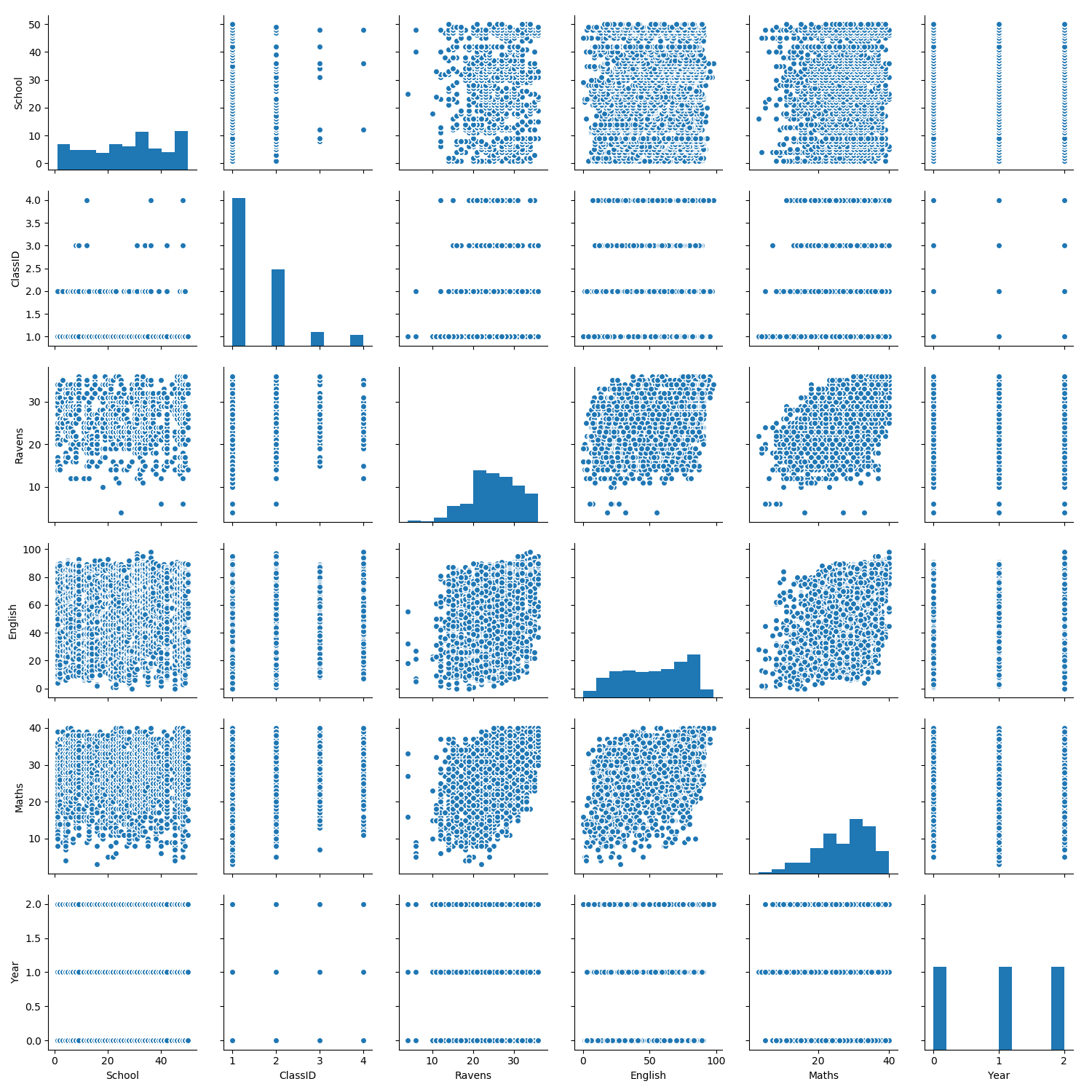
Visualization: Grade at tests in in exams depend on socio-economic status, year at school, …

The simplest way to do this is using seaborn’s pairplot function.

import seaborn as sns
sns.pairplot(exams.drop(columns=['StudentID']))

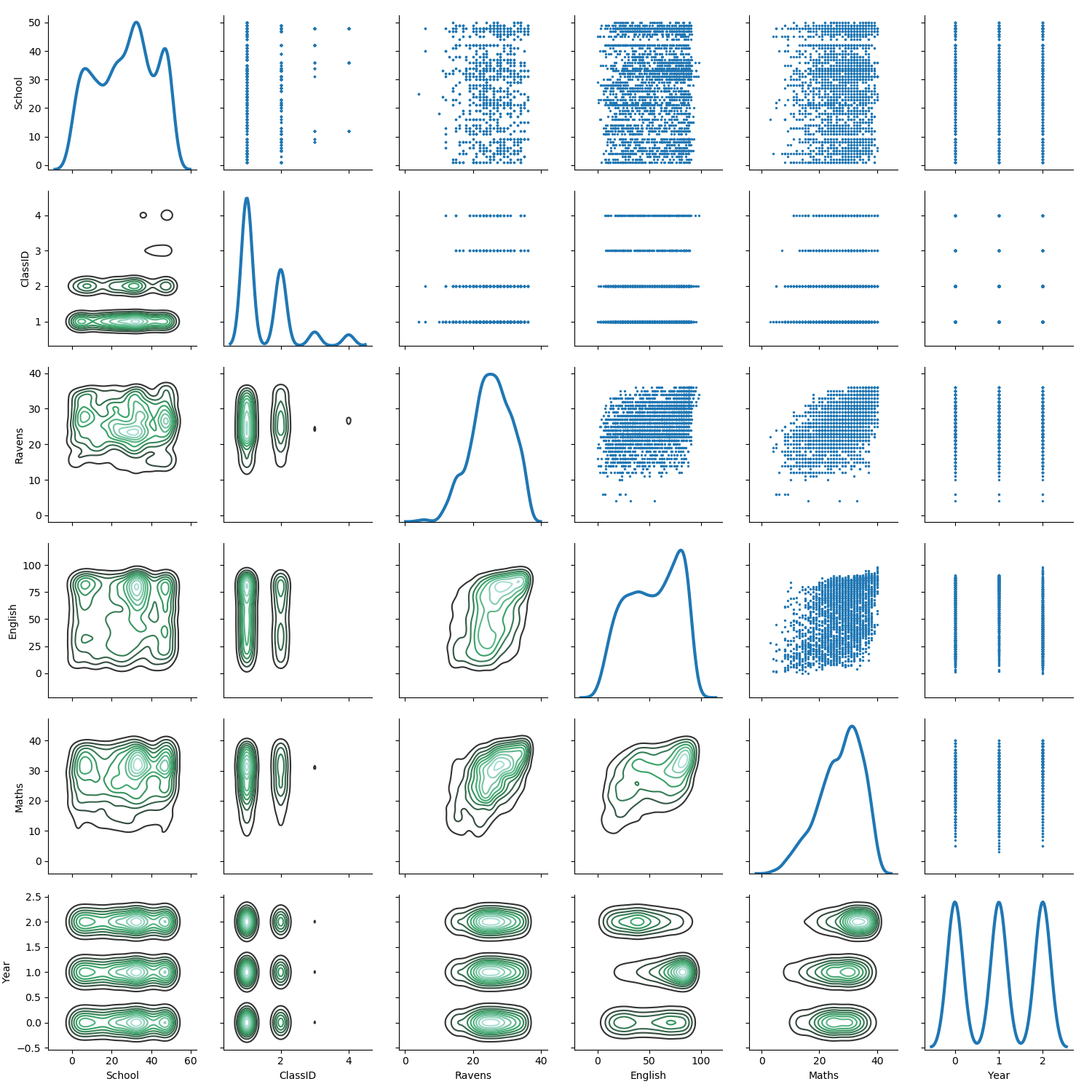
A more elaborate plot using density estimation gives better understanding of the dense regions:

g = sns.PairGrid(exams.drop(columns=['StudentID']),
                 diag_sharey=False)
g.map_lower(sns.kdeplot)
g.map_upper(plt.scatter, s=2)
g.map_diag(sns.kdeplot, lw=3)

Prediction: Can we predict test grades in maths from demographics (ie, not from other grades)?

# A bit of feature engineering to get a numerical matrix (easily done
# with the ColumnTransformer in scikit-learn >= 0.20)
X = exams.drop(columns=['StudentID', 'Maths', 'Ravens', 'English'])
# Encode gender as an integer variables
X['Gender'] = X['Gender'] == 'Girl'
# One-hot encode social class
X = pd.get_dummies(X, drop_first=True)
y = exams['Maths']

from sklearn import ensemble
print(cross_val_score(ensemble.GradientBoostingRegressor(), X, y,
                      cv=10).mean())

Out:

0.0704221342991

We can predict!

But there is one caveat: are we simply learning to recognive students across the years? There is many implicit informations about students: notably in the school ID and the class ID.

Stratification To test for this, we can make sure that we have different students in the train and the test set.

from sklearn import model_selection
cv = model_selection.GroupKFold(10)

print(cross_val_score(ensemble.GradientBoostingRegressor(), X, y,
                      cv=cv, groups=exams['StudentID']).mean())

Out:

0.14218996362

It works better!

The classifier learns better to generalize, probably by learning stronger invariances from the repeated measures on the students

1.2.2.3. Summary

Samples often have a dependency structure, such a with time-series, or with repeated measures. To have a meaningful measure of prediction error, the link between the train and the test set must match the important one for the application. In time-series prediction, it must be in the future. To learn a predictor of the success of an individual from demographics, it might be more relevant to predict across individuals. If the variance across individuals is much larger than the variance across repeated measurement, as in many biomedical applications, the choice of cross-validation strategy may make a huge difference.

Total running time of the script: ( 0 minutes 29.565 seconds)