1.3. Underfit vs overfit: do I need more data, or more complex models?

This is adapted from the scikit-learn chapter in the scipy lectures.

1.3.1. A toy problem: fitting polynomes

1.3.1.1. Data generation model

We consider data generated by the following mechanism, as a toy model of housing prices

import numpy as np

def generating_func(x, err=1):
    return np.random.normal(10 - 1. / (x + 0.1), err)

1.3.1.2. Polynomial regression

The crucial hyperparameter is the degree

from sklearn.pipeline import make_pipeline
from sklearn.preprocessing import PolynomialFeatures
from sklearn.linear_model import LinearRegression
model = make_pipeline(PolynomialFeatures(degree=2), LinearRegression())

1.3.2. Train error versus test error

Generate some data with few samples, for easy understanding

n_samples = 8
np.random.seed(0)
x = 10 ** np.linspace(-2, 0, n_samples)
y = generating_func(x)

# For plotting
x_plot = np.linspace(-0.2, 1.2, 1000)

# randomly sample the data
np.random.seed(1)
x_test = np.random.random(200)
y_test = generating_func(x_test)

1.3.2.1. Underfit: high bias

import matplotlib.pyplot as plt
plt.figure(figsize=(6, 4))
plt.scatter(x, y, marker='x', c='k', s=100)
plt.scatter(x_test, y_test, marker='.', c='k', s=50, alpha=.2)

degree = 1
model = make_pipeline(PolynomialFeatures(degree), LinearRegression())
model.fit(x[:, np.newaxis], y)
plt.plot(x_plot, model.predict(x_plot[:, np.newaxis]), '-b')

plt.xlim(-0.2, 1.2)
plt.ylim(0, 12)
plt.xlabel('house size')
plt.ylabel('price')

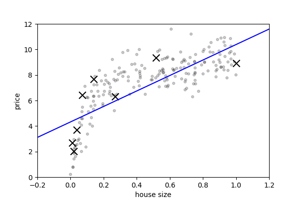
This model has a low train score (high train error):

print(model.score(x[:, np.newaxis], y))

Out:

0.557186529575

If we apply it to the unseen data, the test error is

print(model.score(x_test[:, np.newaxis], y_test))

Out:

0.556942968895

1.3.2.2. Overfit: high variance

plt.figure(figsize=(6, 4))
plt.scatter(x, y, marker='x', c='k', s=100)
plt.scatter(x_test, y_test, marker='.', c='k', s=50, alpha=.2)

degree = 6
model = make_pipeline(PolynomialFeatures(degree), LinearRegression())
model.fit(x[:, np.newaxis], y)
plt.plot(x_plot, model.predict(x_plot[:, np.newaxis]), '-b')

plt.xlim(-0.2, 1.2)
plt.ylim(0, 12)
plt.xlabel('house size')
plt.ylabel('price')

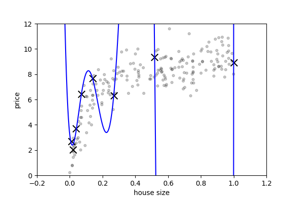
This model has a high train score (very low train error):

print(model.score(x[:, np.newaxis], y))

Out:

0.994643291526

If we apply it to the unseen data, the test error is

print(model.score(x_test[:, np.newaxis], y_test))

Out:

-97767.6303449

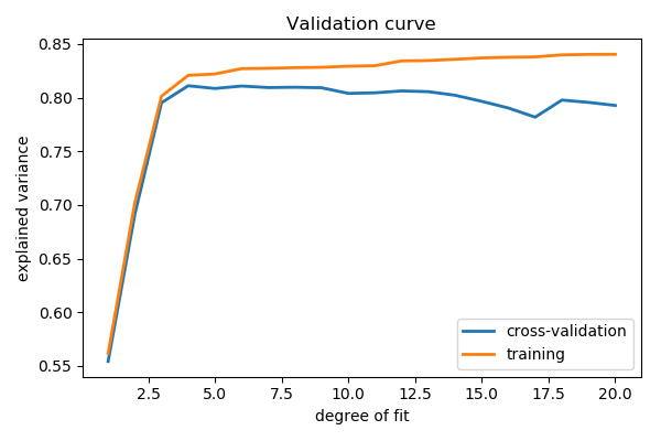
1.3.3. Validation curve varying model complexity

Fit polynomes of different degrees to a dataset: for too small a degree, the model underfits, while for too large a degree, it overfits.

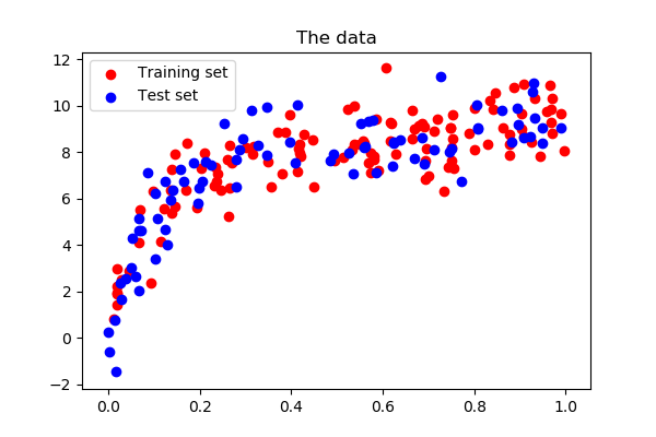
1.3.3.1. Generate a larger dataset

np.random.seed(1)
x = np.random.random(200)
y = generating_func(x)

# split into training, validation, and testing sets.
from sklearn.model_selection import train_test_split
x_train, x_test, y_train, y_test = train_test_split(x, y, test_size=.4)

Show the training and validation sets

plt.figure(figsize=(6, 4))
plt.scatter(x_train, y_train, color='red', label='Training set')
plt.scatter(x_test, y_test, color='blue', label='Test set')
plt.title('The data')
plt.legend(loc='best')

1.3.3.2. The validation_curve function

from sklearn.model_selection import validation_curve

degrees = np.arange(1, 21)
model = make_pipeline(PolynomialFeatures(), LinearRegression())

# The parameter to vary is the "degrees" on the pipeline step
# "polynomialfeatures"
train_scores, validation_scores = validation_curve(
                 model, x[:, np.newaxis], y,
                 param_name='polynomialfeatures__degree',
                 param_range=degrees)

# Plot the mean train error and validation error across folds
plt.figure(figsize=(6, 4))
plt.plot(degrees, validation_scores.mean(axis=1), lw=2,
         label='cross-validation')
plt.plot(degrees, train_scores.mean(axis=1), lw=2, label='training')

plt.legend(loc='best')
plt.xlabel('degree of fit')
plt.ylabel('explained variance')
plt.title('Validation curve')
plt.tight_layout()

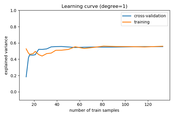
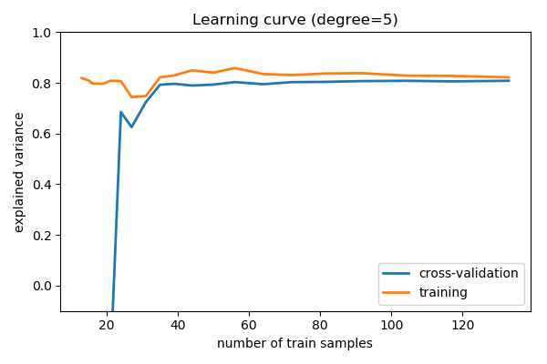
1.3.4. Learning curves: varying the amount of data

Plot train and test error with an increasing number of samples

# A learning curve for d=1, 5, 15
for d in [1, 5, 15]:
    model = make_pipeline(PolynomialFeatures(degree=d), LinearRegression())

    from sklearn.model_selection import learning_curve
    train_sizes, train_scores, validation_scores = learning_curve(
        model, x[:, np.newaxis], y,
        train_sizes=np.logspace(-1, 0, 20))

    # Plot the mean train error and validation error across folds
    plt.figure(figsize=(6, 4))
    plt.plot(train_sizes, validation_scores.mean(axis=1),
            lw=2, label='cross-validation')
    plt.plot(train_sizes, train_scores.mean(axis=1),
                lw=2, label='training')
    plt.ylim(ymin=-.1, ymax=1)

    plt.legend(loc='best')
    plt.xlabel('number of train samples')
    plt.ylabel('explained variance')
    plt.title('Learning curve (degree=%i)' % d)
    plt.tight_layout()

• 
• 
• 

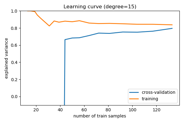
1.3.5. Summary

Comparing train and test error, ideal when vary parameters and amount of data, tells us whether the model is:

• Overfitting, ie data limited, and should not be made more complex and regularization is important, or ideally aquiring more data
• Underfitting, ie not rich enough for the data available, and should be made complex

---

Total running time of the script: ( 0 minutes 1.420 seconds)