I have tagged and released the scikit-learn 0.14 release yesterday evening, after more than 6 months of heavy development from the team. I would like to give a quick overview of the highlights of this release in terms of features but also in term of performance. Indeed, the scikit-learn developers believe that performance matters and strive to be fast and efficient on fairly datasets.
I will show in this article on a couple of benchmarks that we have significant performance improvement and are competitive with the faster libraries such as the proprietary WiseRF.
Prohiminent new features
Most of the new features of the upcoming release have been mentionned more in details on Andy Mueller’s blog. I am just giving a quick list here for completness (see also the full list of changes):
Major new estimators:
- AdaBoost (by Noel Dawe and Gilles Louppe): the classic boosting algorithm. This implementation can be applied to any estimator, but uses trees by default. AdaBoost is a learning strategy that builds from simple learning strategies by focussing successively on samples that are not well predicted. Typically, the simple learners (called weak learners) can be rules as simple as taking simple thresholds of observed quantities (this will form decision stumps). Documentation — Example
- Biclustering (by Kemal Eren): clustering rows and columns of the data matrices. Suppose you have access to the shopping list of many consumers, biclustering would consists is grouping both consumers and product they bought to come up with stories such as “geeks buy computers and phones”, where “geeks” would be a group of consumers and “computers” and “phones” would be groups of products. Documentation — Example
- Missing value imputation (by Nicolas Tresegnie): simple transformer filling missing data with means or medians. If your data-acquisition has failures, human or material, you can easily end up with some descriptors missing for some observations. It would be a pitty to throw away either those observations, or some descriptors. “Imputation” fills in the blanks with simple strategies. Documentation — Example
- RBMs (Restricted Boltzmann Machines) (by Yann Dauphin): a neural network model useful for unsupervised learning of features. Restricted Boltzmann machines learn a set of hidden (latent) factors that have, for each observation, a probability to be activated or not. These activations are found so that they explain the data well, when combined across all the hidden factors with connection weights. Typically, they form a new feature set that can be useful in a prediction task. Documentation — Example
- RandomizedSearchCV (by Andreas Mueller): setting meta-parameters on estimators using a randomized parameter exploration rather than a grid, as in a grid-search. A CV (cross-validated) meta-estimator sets parameters of an estimator by maximizing their cross-validated prediction scores. This entails fitting the estimator for each parameter value tried. The randomized-search explores the parameter space randomly, avoiding the exponential growth in number of points to fit of the grid search. Documentation — Example
Infrastucture work:
- New wesbite (mostly by Gilles Louppe, Nelle Varoquaux, Vincent Michel and Andreas Mueller). The redesign of the website had two objectives: i) unclutter the pages to help prioritize information, ii) make it easier for users to find the stable documentation, if they follow an external link to a documentation of previous releases. I think that it also looks prettier :).
- Python 3 support (Justin Vincent, Lars Buitinck, Subhodeep Moitra and Olivier Grisel). As a side note, under Python 3.3, on Windows, we have found that np.load can trigger segfaults, which means our test suite crashes. The tests not relying on np.load pass.
Major API changes
- The scoring parameter One of the benefits of scikit-learn over other learning packages is that it can set parameters to maximizing a prediction score. However, the prediction that one would want to optimize might depend on the application. Also, some scores can only be computed with specific estimators, for instance because they require probabilistic prediction. Andreas Mueller and Lars Buitinck came up with a new API to specifies the scoring strategy that is versatile and hides complexity from the user. This replaces the score_func argument.
- *sklearn.test()* is deprecated and will not run the test suite. Please use nosetests sklearn from the command line.
The full list of API changes can be found on the change log.
Performance improvements
Many part of the codebase got speed-ups, with a focus on making scikit-learn more scalable for bigger data.
- The trees (random forests and extra-trees) were massively sped up by Gilles Louppe, bringing them to par with the fastest libraries (see benchmarks below)
- Jake Vanderplas improved the BallTree and implemented fast KDTrees for nearest-neighbor search (benchmarks below).
- “cleverless” made the DBSCAN implementation scale to a large number of samples by relying on KDTree and BallTree for neighbor search.
- KMeans much faster on sparse data (Lars Buitinck)
- For text vectorization: much faster CountVectorizer and TfidVectorizer with less memory consumption (Jochen Wersdorfer and Roman Sinayev)
- Out-of-core learning for discrete naive Bayes classifiers by Olivier Grisel. Estimators that implement a partial_fit method can be used to fit the model with an out-of-core strategy, as illustrated by the out-of-core classification example. These settings are well suited to very big data.
- FastICA: less memory consumptions and slightly faster code (Denis Engemann and Alexandre Gramfort)
- Faster IsotonicRegression (Nelle Varoquaux)
- OrthogonalMatchingPursuitCV by Alexandre Gramfort and Vlad Niculae: while strictly-speaking not a speedup of a existing estimator, this new estimator means that OMP parameters can be set much faster.
We are faster: lies, damn lies and benchmarks
“There are three kinds of lies: lies, damned lies and statistics.” —
Mark Twain’s Own Autobiography: The Chapters from the North American Review
I claim we have gotten faster at certain things. Other libraries, such as WiseRf, have performance claims compared to us. It turns out that benching statistical learning code is very hard, because speed depends a lot on the properties of the data.
Fast neighbor searches: good KDTrees beat BallTrees
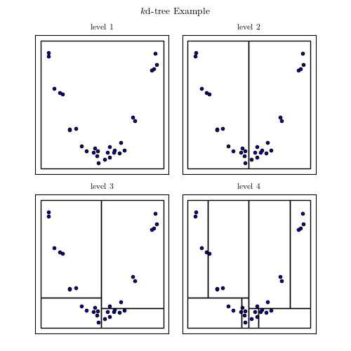
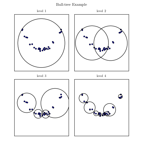
A good example of interplay between properties of the data and computational speed is the nearest neighbor search. In general, finding the nearest neighbor to a point out of n other points will cost you n operations, as you have to compute the distance to each of these points. However, building a tree-like data structure ahead of time can make this query cost only log n. If these points are in 1D, ie simple scalars, this would be achieve by sorting them. In higher dimensions that can be achieved by building a KDTree, made of planes dividing the space in half-spaces, or a BallTree, made of nested balls.

KD Tree Image from AstroML’s documentation

Ball tree Image from AstroML’s documentation
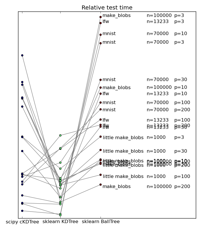
Popular wisdom in machine learning is that in high dimensions, BallTrees scale better than KDTrees. This is explained by the fact that as the dimensionality grows, the number of planes required to break up the space grows too. On the contrary, if the data has structure, BallTrees can more efficiently cover this structure. I have benched scikit-learn’s KDTree and BallTree, as well as scipy’s KDTree, which employs a simpler tree-building strategy, on a variety of datasets, both real-life and artificial. Below if a summary plot giving relative performance of neighbor search

n is the number of data points, and p the dimensionality.
We can see that no approach win on all counts. That said, it came to a surprise to me to see that even in high dimension, scikit-learn’s KDTree outperformed the BallTrees. This is explained because these datasets do not display a heavily-structured low ambient dimension. On highly-structured synthetic data, the benefit of BallTree can clearly stand out, as shown by Jake here. However, on most dataset people encounter, it seems that this is not the case. Note also that scikit-learn’s KDTree tend to scale better in high dimension than scipy’s. This is due to the more elaborate choice of cutting planes. Note that it also has a cost, and may backfire, as on some datasets scikit-learn is slower than scipy.
Overall, the new KDTree in scikit-learn seem to be giving an excellent compromise. Congratulations Jake!
DBSCAN is faster with trees
DBSCAN is a clustering algorithm that relies heavily on the local neighborhood structure. The implementation in scikit-learn 0.13 computed the complete n by n matrix of distance between observations, which means that if you had a lot of data, you would blow your memory. In the 0.14 release, DBSCAN uses the BallTree, and as a result scales to much larger datasets and brings speed benefits. Here is a comparison between 0.13 and 0.14 implementations (I couldn’t put data as large as I wanted because the 0.13 code would blow):
| Dataset | time with 0.13 | time with 0.14 |
|---|---|---|
| “lfw”: 13233 samples, 5 features | 6.57 seconds | 3.59 seconds |
| “make_blobs”: 30000, with 10 features | 33.50 seconds | 12.87 seconds |
Importantly, the scaling is different: while the 0.13 code scales as n ^ 2, the 0.14 code scales as n log n. This means that the benefit is bigger for large dataset.
Scikit-learn 0.14’s random forests are fast
Gilles Louppe has made the random forests significantly faster in the 0.14 release. Let us bench them in comparison with WiseIO’s WiseRf, a proprietary package that only does random forest and for which the main selling point is that it is significantly than scikit-learn. However, let us also bench ExtraTrees, a tree-based model that is very similar to random forests, but that in our experience can be implemented a bit faster, and tends to work better.
On the digits dataset (1797 samples, 641 features):
| Forest implementation | train time | test time | prediction accuracy |
| Sklearn ExtraTrees | 2.641s | 0.082s | 0.986 |
| Sklearn RandomForest | 5.074s | 0.088s | 0.981 |
| WiseRF | 5.665s | 0.108s | 0.979 |
So we see that on a mid-sized dataset, scikit-learn is faster than WiseRF, and ExtraTrees is twice as fast as RandomForest, for better results.
On the MNIST dataset (70000 samples, 784 features):
| Forest implementation | train time | test time | prediction accuracy |
| Sklearn ExtraTrees | 1378.141s | 4.768s | 0.976 |
| Sklearn RandomForest | 1639.866s | 4.132s | 0.972 |
| WiseRF | 1102.465s | 14.542s | 0.972 |
On a big dataset, WiseRF takes the lead, but not by a large factor.
Using 2 CPUs (n_jobs=2) on the digits dataset:
| Forest implementation | train time | test time | prediction accuracy |
| Sklearn ExtraTrees | 4.874s | 1.478s | 0.986 |
| Sklearn RandomForest | 5.716s | 1.349s | 0.978 |
| WiseRF | 3.264s | 0.104s | 0.979 |
Both scikit-learn and WiseRF can use several CPUs. However, the Python parallel execution model via multiple processes has an overhead in term of computing time and of memory usage. The internals of WiseRF are coded in C++, and thus it is not limited by this overhead. Also, because of the memory duplication with multiples processes in scikit-learn, I could not run it on MNIST with 2 jobs. Next release will address these issues, partly by using memmapped arrays to share memory between processes.
We make good use of funding: the Paris sprint
A couple of weeks ago, we had a coding sprint in Paris. We were able to bring in a lot of core developers from all over Europe thanks to our sponsors: FNRS, AFPy, Telecom Paristech, and Saint-Gobain Recherche. The total budget, including accommodation and travel, was a couple thousand euros, thanks to Telecom Paristech and tinyclues helping us with accommodation and hosting the sprint.
The productivity of such a sprint is huge, both because we get together and work efficiently, but also because we get back home and keep working (I have been sleep deprived because of late-night hacking ever since the sprint). As an illustration, here is the diagram of commits as can be seen on Github. The huge spike correspond to the second international sprint: Paris 2013.

We now have a “donate” button on the website. I can assure you that your donations are well spent and turned into code.
