PCA and ICA: Identifying combinations of variables

Dimension reduction with PCA

If we have three-dimensional data, for instance simultaneous measurements made by three thermometers positioned at different locations in a room. The data forms a cluster of points in a 3D space:

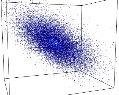
If the temperature in that room is conditioned by only two parameters, the setting of a heater and the outside temperature, we probably have too much data: the three sets of measurements can be expressed as a linear combination of two fluctuating variable, and an additional much smaller noise parameter. In other words, the data mostly lies in a 2D plane embedded in the 3D measurement space.

We can use PCA (Principal Component Analysis) to find this plane: PCA will give us the orthogonal basis in which the covariance matrix of our data is diagonal. The vectors of this basis point in successive orthogonal directions in which the data variance is maximum. In the case of data mainly residing on a 2D plane, the variance is much greater along the two first vectors, which define our plane of interest, than along the third one:

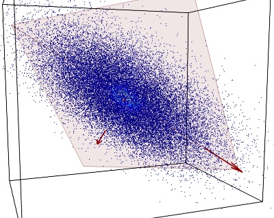
The covariance eigenvectors identified by PCA are shown in red. The plane defined by the 2 largest eigenvectors is shown in light red.

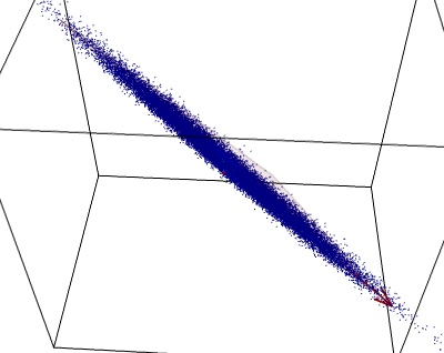
If we look at the data in the plane identified by PCA, it is clear that it was mostly 2D:

Understanding PCA with a Gaussian model

Let x and y be two normal-distributed variables, describing the processes we are observing:

and

Let a and b be two observation variables, linear combinations of x and y:

and

PCA is performed by applying an SVD (singular value decomposition) on the observed data matrix:

This is equivalent to find the eigenvalues and eigenvectors of Y^TY, the correlation matrix of the observed data. The multidimensional (or multivariate, in statistical jargon) probability density function of Y is written:

where r is the position is the (a,b) observation space, and M the correlation matrix. Diagonalizing the matrix M corresponds to finding a rotation matrix U such that:

With S a diagonal matrix. In other words, U is a rotation of the observation space to change to a basis where the probability density function is written:

In this new basis, Y can thus be interpreted as a sum of independent normal processes of different variance.

We can thus picture the PCA as a way of finding independent normal processes. The different steps of the argument exposed above can be pictured in the following figure:

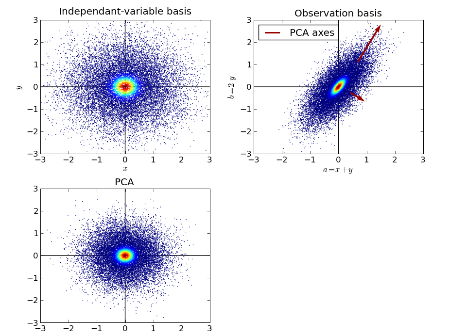
First we represent samples drawn from x and y in their original space, the basis of the independent variables. Then we represent the (a, b) samples, and we apply PCA on these samples, to estimate the eigenvectors of the covariance matrix. Then we represent the data projected in the basis estimated by PCA. One important detail to note, is that after PCA, the data is most often rescaled: each direction is divided by the corresponding sample standard deviation identified by PCA. After this operation, all directions of space play the same role, the data is spheric, or “white”.

PCA was able to identify the original independent variables x and y in the a and b samples only because they were mixed with different variance. For a isotropic Gaussian model, any basis can describe the data in terms of independent normal process.

PCA on non normal data

More generally, the PCA algorithm can be understood as an algorithm finding the direction of space with the highest sample variance, and moving on to the orthogonal subspace of this direction to find the next highest variance, and iteratively discovering an ordered orthogonal basis of highest variance. This is well adapted to normal processes, as their covariance is indeed diagonal in an orthogonal basis. In addition, the resulting vectors come with a “PCA score”, ie the variance of the data projected along the direction they define. Thus when using PCA for dimension reduction, we can choose the subspace defined by the first n PCA vectors, on the basis that they explain a given percentage of the variance, and that the subspace they define is the subspace of dimension n that explains the largest possible fraction of the total variance.

However, on strongly non-Gaussian processes, the variance may not be the quantity of interest.

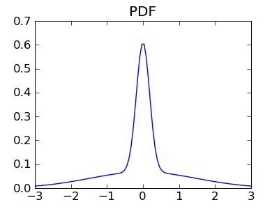
Let us consider the same model as above, with two independent variables x and y thought with strongly non-Gaussian distributions. Here we use a mixture of a narrow Gaussian, and wide one, to populate the tails:

We can apply the same operations on these random variables: change of basis to an observation basis made of a and b, and PCA on the resulting sample:

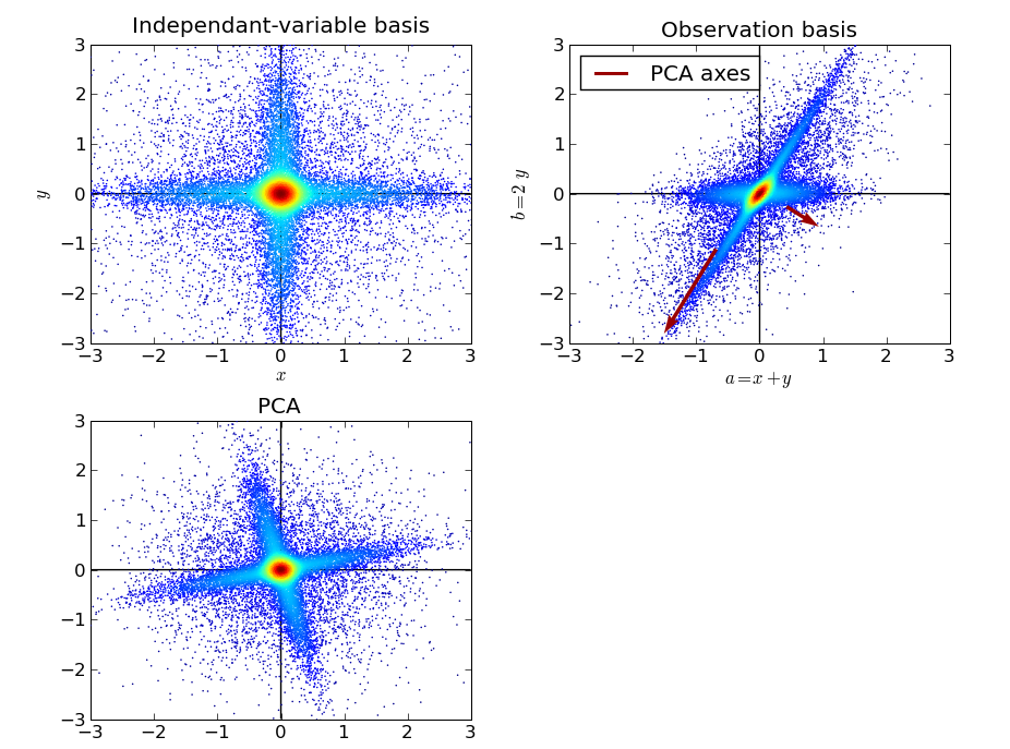
We can see that the PCA did not properly identify the original independent variables. The variance criteria is not good-enough when the principle axis of the observed distribution are not orthogonal, as the highest variance can be found in a direction mixing the two process. Indeed the largest PCA direction is found slightly off axis. In addition the second direction can only be found orthogonal to the first one, as this is a restriction of PCA.

On the other side, the data after PCA is much more spheric than the original data. No strong anisotropy is found in the central part of the sample cloud, which contributes most to the variance.

ICA: independent, non-Gaussian variables

For strongly non-Gaussian processes, the above example shows that separating independent process should be done by looking at fine details of the distribution, such as the tails. Indeed, after PCA, the Gaussian part of the processes have been separated by their variance, and the resulting, rescaled, samples cannot be decomposed in independent process in a Gaussian model, as they all have the same variance, and would already be considered independent under a Gaussian hypothesis.

A popular class of algorithms to separate independent sources, called ICA (independent component analysis) makes the simplification that finding independent sources out of such data can be reduced to finding maximally non-Gaussian. Indeed, the central-limit theorem tells us that the sum of non-Gaussian processes lead to Gaussian process. Conversely, with equal variance multivariate samples, the more non-Gaussian a signal extracted from the data, the less independent -and non-Gaussian- variables it contains.

A good discussion of these arguments can be found in following paper: http://www.cis.hut.fi/aapo/papers/IJCNN99_tutorialweb/IJCNN99_tutorial3.html

ICA is thus an optimization algorithm that from the data extracts the direction with the least-Gaussian PDF, removes the data explained by this variable from the signal, and iterates.

Applying ICA to the previous model yields the following:

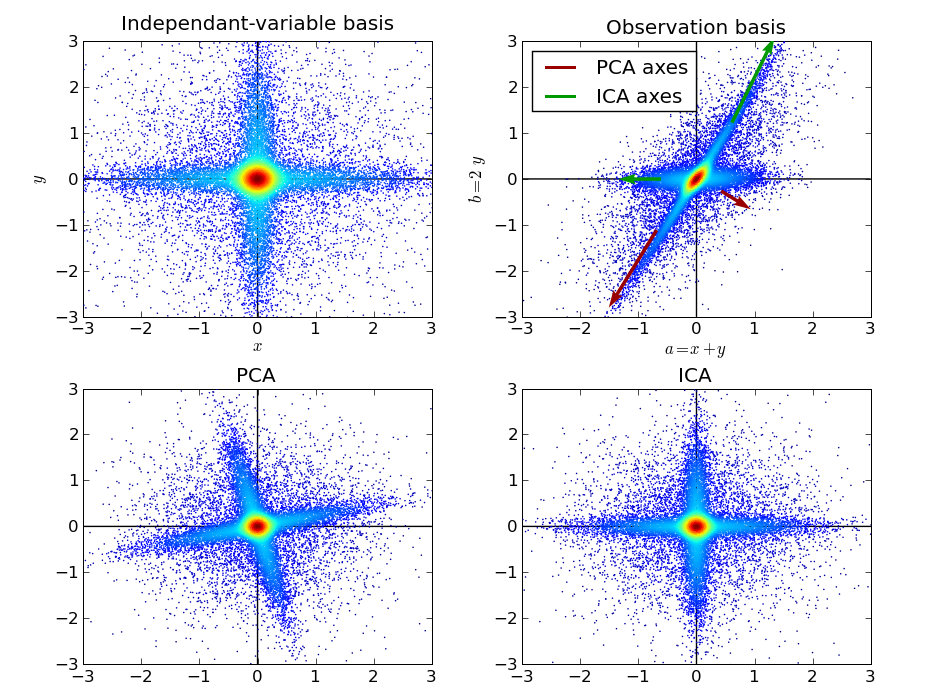
We can see that ICA has well identified the original independent data variables. Its use of the tails of the distribution was paramount for this task. In addition, ICA relaxes the constraint that all identified directions must be perpendicular. This flexibility was also important to match our data.