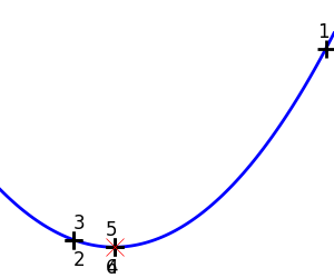
2.7.4.8. Brent’s method

Illustration of 1D optimization: Brent’s method

• 
• 
• 
• 

Out:

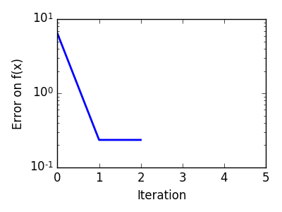
('Converged at ', 6)
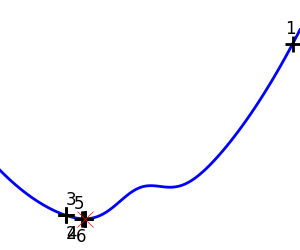
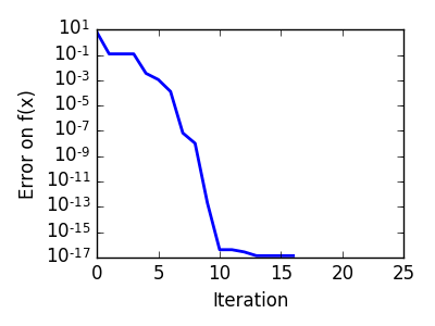
('Converged at ', 23)

import numpy as np
import pylab as pl
from scipy import optimize

x = np.linspace(-1, 3, 100)
x_0 = np.exp(-1)

def f(x):
    return (x - x_0)**2 + epsilon*np.exp(-5*(x - .5 - x_0)**2)

for epsilon in (0, 1):
    pl.figure(figsize=(3, 2.5))
    pl.axes([0, 0, 1, 1])

    # A convex function
    pl.plot(x, f(x), linewidth=2)

    # Apply brent method. To have access to the iteration, do this in an
    # artificial way: allow the algorithm to iter only once
    all_x = list()
    all_y = list()
    for iter in range(30):
        result = optimize.minimize_scalar(f, bracket=(-5, 2.9, 4.5), method="Brent",
                    options={"maxiter": iter}, tol=np.finfo(1.).eps)
        if result.success:
            print('Converged at ', iter)
            break

        this_x = result.x
        all_x.append(this_x)
        all_y.append(f(this_x))
        if iter < 6:
            pl.text(this_x - .05*np.sign(this_x) - .05,
                    f(this_x) + 1.2*(.3 - iter % 2), iter + 1,
                    size=12)

    pl.plot(all_x[:10], all_y[:10], 'k+', markersize=12, markeredgewidth=2)

    pl.plot(all_x[-1], all_y[-1], 'rx', markersize=12)
    pl.axis('off')
    pl.ylim(ymin=-1, ymax=8)

    pl.figure(figsize=(4, 3))
    pl.semilogy(np.abs(all_y - all_y[-1]), linewidth=2)
    pl.ylabel('Error on f(x)')
    pl.xlabel('Iteration')
    pl.tight_layout()

pl.show()

Total running time of the script: ( 0 minutes 0.533 seconds)