3.6.9.14. The eigenfaces example: chaining PCA and SVMs

The goal of this example is to show how an unsupervised method and a supervised one can be chained for better prediction. It starts with a didactic but lengthy way of doing things, and finishes with the idiomatic approach to pipelining in scikit-learn.

Here we’ll take a look at a simple facial recognition example. Ideally, we would use a dataset consisting of a subset of the Labeled Faces in the Wild data that is available with sklearn.datasets.fetch_lfw_people(). However, this is a relatively large download (~200MB) so we will do the tutorial on a simpler, less rich dataset. Feel free to explore the LFW dataset.

from sklearn import datasets
faces = datasets.fetch_olivetti_faces()
faces.data.shape

Let’s visualize these faces to see what we’re working with

from matplotlib import pyplot as plt
fig = plt.figure(figsize=(8, 6))
# plot several images
for i in range(15):
    ax = fig.add_subplot(3, 5, i + 1, xticks=[], yticks=[])
    ax.imshow(faces.images[i], cmap=plt.cm.bone)

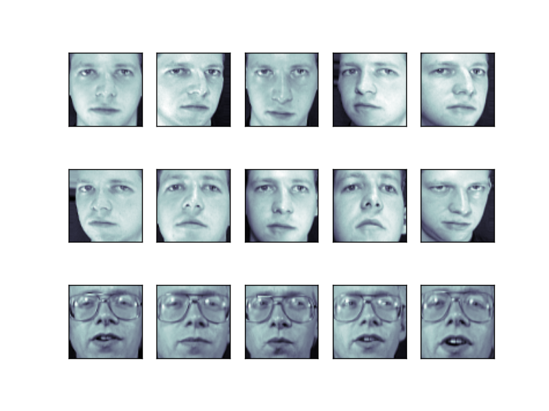
Tip

Note is that these faces have already been localized and scaled to a common size. This is an important preprocessing piece for facial recognition, and is a process that can require a large collection of training data. This can be done in scikit-learn, but the challenge is gathering a sufficient amount of training data for the algorithm to work. Fortunately, this piece is common enough that it has been done. One good resource is OpenCV, the Open Computer Vision Library.

We’ll perform a Support Vector classification of the images. We’ll do a typical train-test split on the images:

from sklearn.model_selection import train_test_split
X_train, X_test, y_train, y_test = train_test_split(faces.data,
        faces.target, random_state=0)

print(X_train.shape, X_test.shape)

Out:

((300, 4096), (100, 4096))

Preprocessing: Principal Component Analysis

1850 dimensions is a lot for SVM. We can use PCA to reduce these 1850 features to a manageable size, while maintaining most of the information in the dataset.

from sklearn import decomposition
pca = decomposition.PCA(n_components=150, whiten=True)
pca.fit(X_train)

One interesting part of PCA is that it computes the “mean” face, which can be interesting to examine:

plt.imshow(pca.mean_.reshape(faces.images[0].shape),
           cmap=plt.cm.bone)

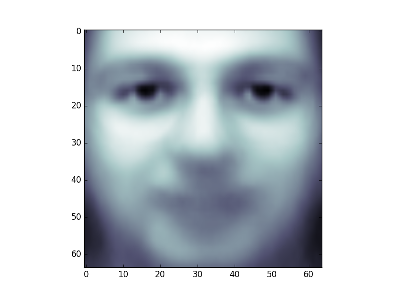
The principal components measure deviations about this mean along orthogonal axes.

print(pca.components_.shape)

Out:

(150, 4096)

It is also interesting to visualize these principal components:

fig = plt.figure(figsize=(16, 6))
for i in range(30):
    ax = fig.add_subplot(3, 10, i + 1, xticks=[], yticks=[])
    ax.imshow(pca.components_[i].reshape(faces.images[0].shape),
              cmap=plt.cm.bone)

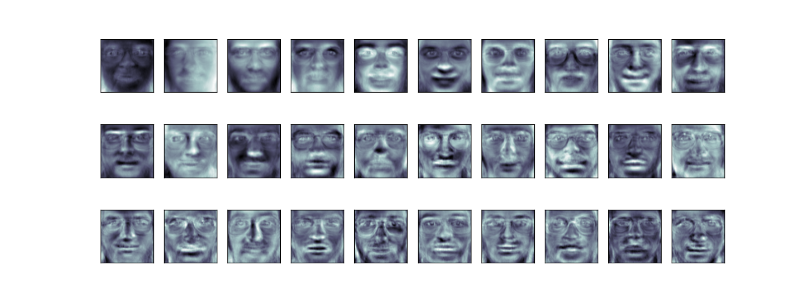
The components (“eigenfaces”) are ordered by their importance from top-left to bottom-right. We see that the first few components seem to primarily take care of lighting conditions; the remaining components pull out certain identifying features: the nose, eyes, eyebrows, etc.

With this projection computed, we can now project our original training and test data onto the PCA basis:

X_train_pca = pca.transform(X_train)
X_test_pca = pca.transform(X_test)
print(X_train_pca.shape)

Out:

(300, 150)

print(X_test_pca.shape)

Out:

(100, 150)

These projected components correspond to factors in a linear combination of component images such that the combination approaches the original face.

Doing the Learning: Support Vector Machines

Now we’ll perform support-vector-machine classification on this reduced dataset:

from sklearn import svm
clf = svm.SVC(C=5., gamma=0.001)
clf.fit(X_train_pca, y_train)

Finally, we can evaluate how well this classification did. First, we might plot a few of the test-cases with the labels learned from the training set:

import numpy as np
fig = plt.figure(figsize=(8, 6))
for i in range(15):
    ax = fig.add_subplot(3, 5, i + 1, xticks=[], yticks=[])
    ax.imshow(X_test[i].reshape(faces.images[0].shape),
              cmap=plt.cm.bone)
    y_pred = clf.predict(X_test_pca[i, np.newaxis])[0]
    color = ('black' if y_pred == y_test[i] else 'red')
    ax.set_title(faces.target[y_pred],
                 fontsize='small', color=color)

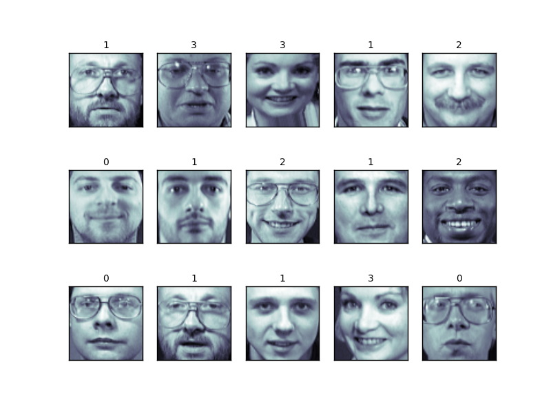
The classifier is correct on an impressive number of images given the simplicity of its learning model! Using a linear classifier on 150 features derived from the pixel-level data, the algorithm correctly identifies a large number of the people in the images.

Again, we can quantify this effectiveness using one of several measures from sklearn.metrics. First we can do the classification report, which shows the precision, recall and other measures of the “goodness” of the classification:

from sklearn import metrics
y_pred = clf.predict(X_test_pca)
print(metrics.classification_report(y_test, y_pred))

Out:

precision    recall  f1-score   support

          0       1.00      0.67      0.80         6
          1       1.00      1.00      1.00         4
          2       0.50      1.00      0.67         2
          3       1.00      1.00      1.00         1
          4       0.50      1.00      0.67         1
          5       1.00      1.00      1.00         5
          6       1.00      1.00      1.00         4
          7       1.00      0.67      0.80         3
          9       1.00      1.00      1.00         1
         10       1.00      1.00      1.00         4
         11       1.00      1.00      1.00         1
         12       1.00      1.00      1.00         2
         13       1.00      1.00      1.00         3
         14       1.00      1.00      1.00         5
         15       0.75      1.00      0.86         3
         17       1.00      1.00      1.00         6
         19       1.00      1.00      1.00         4
         20       1.00      1.00      1.00         1
         21       1.00      1.00      1.00         1
         22       1.00      1.00      1.00         2
         23       1.00      1.00      1.00         1
         24       1.00      1.00      1.00         2
         25       1.00      0.50      0.67         2
         26       1.00      0.75      0.86         4
         27       1.00      1.00      1.00         1
         28       0.67      1.00      0.80         2
         29       1.00      1.00      1.00         3
         30       1.00      1.00      1.00         4
         31       1.00      1.00      1.00         3
         32       1.00      1.00      1.00         3
         33       1.00      1.00      1.00         2
         34       1.00      1.00      1.00         3
         35       1.00      1.00      1.00         1
         36       1.00      1.00      1.00         3
         37       1.00      1.00      1.00         3
         38       1.00      1.00      1.00         1
         39       1.00      1.00      1.00         3

avg / total       0.97      0.95      0.95       100

Another interesting metric is the confusion matrix, which indicates how often any two items are mixed-up. The confusion matrix of a perfect classifier would only have nonzero entries on the diagonal, with zeros on the off-diagonal:

print(metrics.confusion_matrix(y_test, y_pred))

Out:

[[4 0 0 ..., 0 0 0]
 [0 4 0 ..., 0 0 0]
 [0 0 2 ..., 0 0 0]
 ...,
 [0 0 0 ..., 3 0 0]
 [0 0 0 ..., 0 1 0]
 [0 0 0 ..., 0 0 3]]

Pipelining

Above we used PCA as a pre-processing step before applying our support vector machine classifier. Plugging the output of one estimator directly into the input of a second estimator is a commonly used pattern; for this reason scikit-learn provides a Pipeline object which automates this process. The above problem can be re-expressed as a pipeline as follows:

from sklearn.pipeline import Pipeline
clf = Pipeline([('pca', decomposition.PCA(n_components=150, whiten=True)),
                ('svm', svm.LinearSVC(C=1.0))])

clf.fit(X_train, y_train)

y_pred = clf.predict(X_test)
print(metrics.confusion_matrix(y_pred, y_test))
plt.show()

Out:

[[2 0 0 ..., 0 0 0]
 [0 4 0 ..., 0 0 0]
 [0 0 1 ..., 0 0 0]
 ...,
 [0 0 0 ..., 3 0 0]
 [0 0 0 ..., 0 1 0]
 [0 0 0 ..., 0 0 3]]

A Note on Facial Recognition

Here we have used PCA “eigenfaces” as a pre-processing step for facial recognition. The reason we chose this is because PCA is a broadly-applicable technique, which can be useful for a wide array of data types. Research in the field of facial recognition in particular, however, has shown that other more specific feature extraction methods are can be much more effective.

Total running time of the script: ( 0 minutes 3.876 seconds)