Predicting sepsis in the ICU

We predict, from just the first 24 hours of a patient’s ICU stay, whether they will later be diagnosed with sepsis, using a small number of covariates: age, sex, the delay between hospital and ICU admission, and diastolic blood pressure. We compare a linear and a non-linear model, and look at partial dependence plots to understand how the non-linear model uses these covariates to predict.

Learning objectives and take home messages

This notebook introduces a health dataset and develops intuitions on predictive models on this dataset.

Load the PhysioNet sepsis dataset

This dataset was built from the PhysioNet/Computing in Cardiology Challenge 2019, a public dataset of 40,336 ICU patients:

import pandas as pd
df = pd.read_csv("physionet_sepsis.csv")

Data overview

from skrub import TableReport
TableReport(df)

Please enable javascript

The skrub table reports need javascript to display correctly. If you are displaying a report in a Jupyter notebook and you see this message, you may need to re-execute the cell or to trust the notebook (button on the top right or "File > Trust notebook").

This is already a small, curated set of covariates - age, sex, the delay before ICU admission, and diastolic blood pressure:

X = df.drop(columns=["sepsis"])
y = df["sepsis"]

print("Covariates used:", X.columns.tolist())
print("Sepsis rate:", y.mean())

Covariates used: ['age', 'sex', 'hours_before_icu', 'diastolic_bp_mmhg']
Sepsis rate: 0.04052146688223369

Model fitting and prediction

Train / test split

Before fitting models, we split train and test data, in order to have untouched hold-out data (“test”) to evaluate the model. We stratify the split: sepsis is rare in this cohort (~4%).

from sklearn.model_selection import train_test_split

X_train, X_test, y_train, y_test = train_test_split(
    X, y, test_size=0.2, stratify=y, random_state=0
)

Fit a linear model: logistic regression

We use a LogisticRegression from scikit-learn, wrapped in a tabular_pipeline from skrub that does some data preparation.

from sklearn.linear_model import LogisticRegression
from skrub import tabular_pipeline

model_linear = tabular_pipeline(LogisticRegression())
model_linear.fit(X_train, y_train)

Pipeline(steps=[('tablevectorizer',
                 TableVectorizer(datetime=DatetimeEncoder(periodic_encoding='spline'))),
                ('simpleimputer', SimpleImputer(add_indicator=True)),
                ('squashingscaler', SquashingScaler(max_absolute_value=5)),
                ('logisticregression', LogisticRegression())])

In a Jupyter environment, please rerun this cell to show the HTML representation or trust the notebook.
On GitHub, the HTML representation is unable to render, please try loading this page with nbviewer.org.

Evaluate the model on held-out data

from sklearn.metrics import roc_auc_score

y_pred_proba_linear = model_linear.predict_proba(X_test)[:, 1]
auc_linear = roc_auc_score(y_test, y_pred_proba_linear)
print(f"Held-out AUC, linear model (logistic regression): {auc_linear:.3f}")

Held-out AUC, linear model (logistic regression): 0.595

Fit a non-linear model: gradient boosting

This is skrub’s default classification pipeline: a TableVectorizer followed by a HistGradientBoostingClassifier.

model_nonlinear = tabular_pipeline("classifier")
model_nonlinear.fit(X_train, y_train)

Pipeline(steps=[('tablevectorizer',
                 TableVectorizer(low_cardinality=ToCategorical())),
                ('histgradientboostingclassifier',
                 HistGradientBoostingClassifier())])

In a Jupyter environment, please rerun this cell to show the HTML representation or trust the notebook.
On GitHub, the HTML representation is unable to render, please try loading this page with nbviewer.org.

Evaluate it on held-out data

y_pred_proba_nonlinear = model_nonlinear.predict_proba(X_test)[:, 1]
auc_nonlinear = roc_auc_score(y_test, y_pred_proba_nonlinear)
print(f"Held-out AUC, non-linear model (gradient boosting): {auc_nonlinear:.3f}")

Held-out AUC, non-linear model (gradient boosting): 0.660

The non-linear model predicts distinctly better than the linear one, with only four covariates. Let’s now see what drives this prediction.

Model inspection: how do the models predict

Permutation importance: finding the important variables

We use permutation importance to see which variables drive the prediction.

For the linear model

from sklearn.inspection import permutation_importance

perm_linear = permutation_importance(
    model_linear, X_test, y_test, scoring="roc_auc", n_repeats=10, random_state=0
)

importances_linear = pd.DataFrame({
    "feature": X_test.columns,
    "importance_mean": perm_linear.importances_mean,
}).sort_values("importance_mean", ascending=False)

print("Permutation importance (drop in prediction performance when a feature is shuffled):")
print(importances_linear.to_string(index=False))

Permutation importance (drop in prediction performance when a feature is shuffled):
          feature  importance_mean
diastolic_bp_mmhg         0.054677
 hours_before_icu         0.021333
              sex         0.007222
              age        -0.000185

For the non-linear model

perm_nonlinear = permutation_importance(
    model_nonlinear, X_test, y_test, scoring="roc_auc", n_repeats=10, random_state=0
)

importances_nonlinear = pd.DataFrame({
    "feature": X_test.columns,
    "importance_mean": perm_nonlinear.importances_mean,
}).sort_values("importance_mean", ascending=False)

print("Permutation importance (drop in prediction performance when a feature is shuffled):")
print(importances_nonlinear.to_string(index=False))

Permutation importance (drop in prediction performance when a feature is shuffled):
          feature  importance_mean
 hours_before_icu         0.131079
diastolic_bp_mmhg         0.046590
              age         0.011812
              sex        -0.001744

Delay before ICU admission stands out as an important predictor of sepsis. Let’s now understand how it relates to the risk of sepsis.

Partial dependence on delay before ICU admission

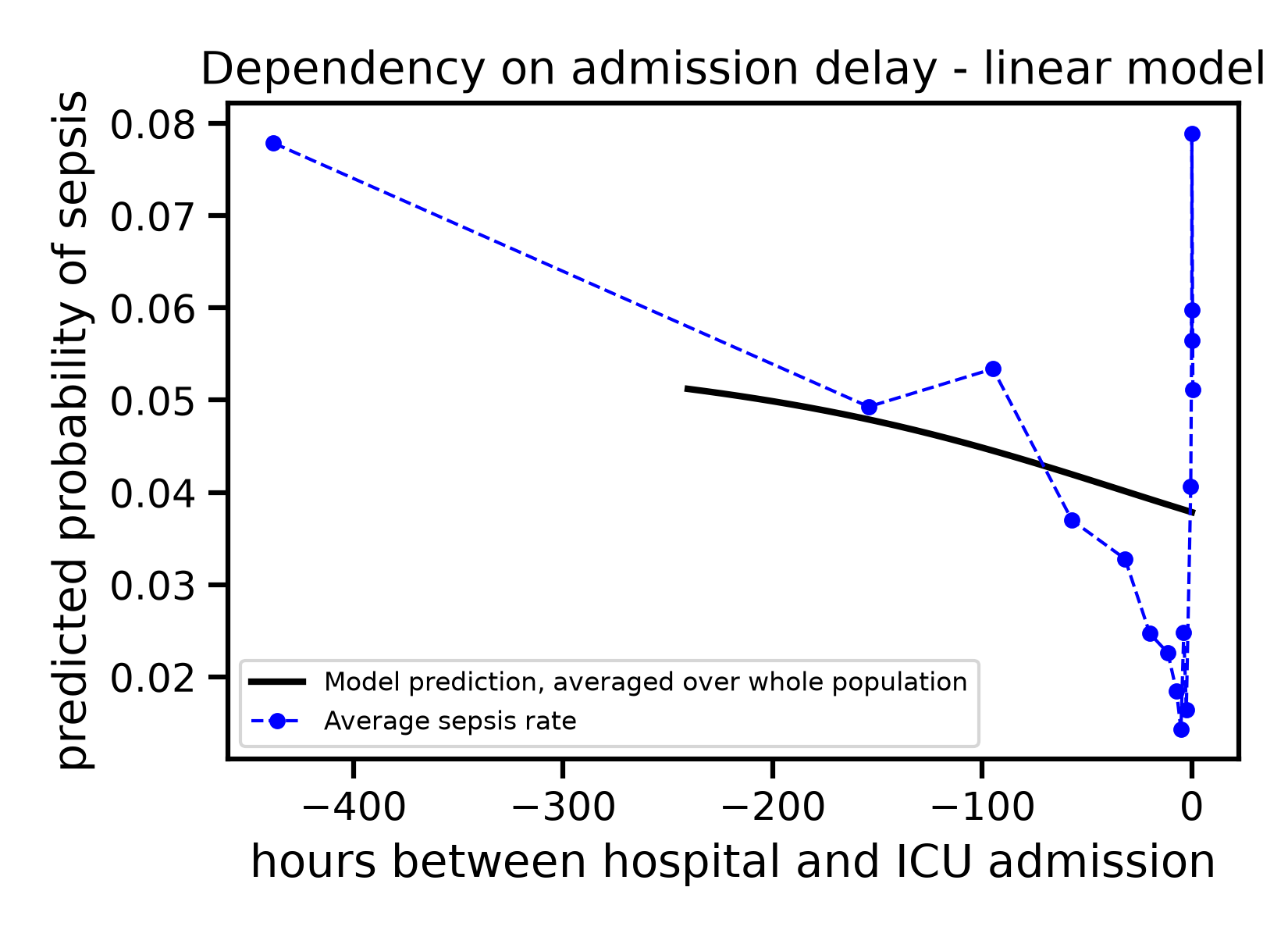
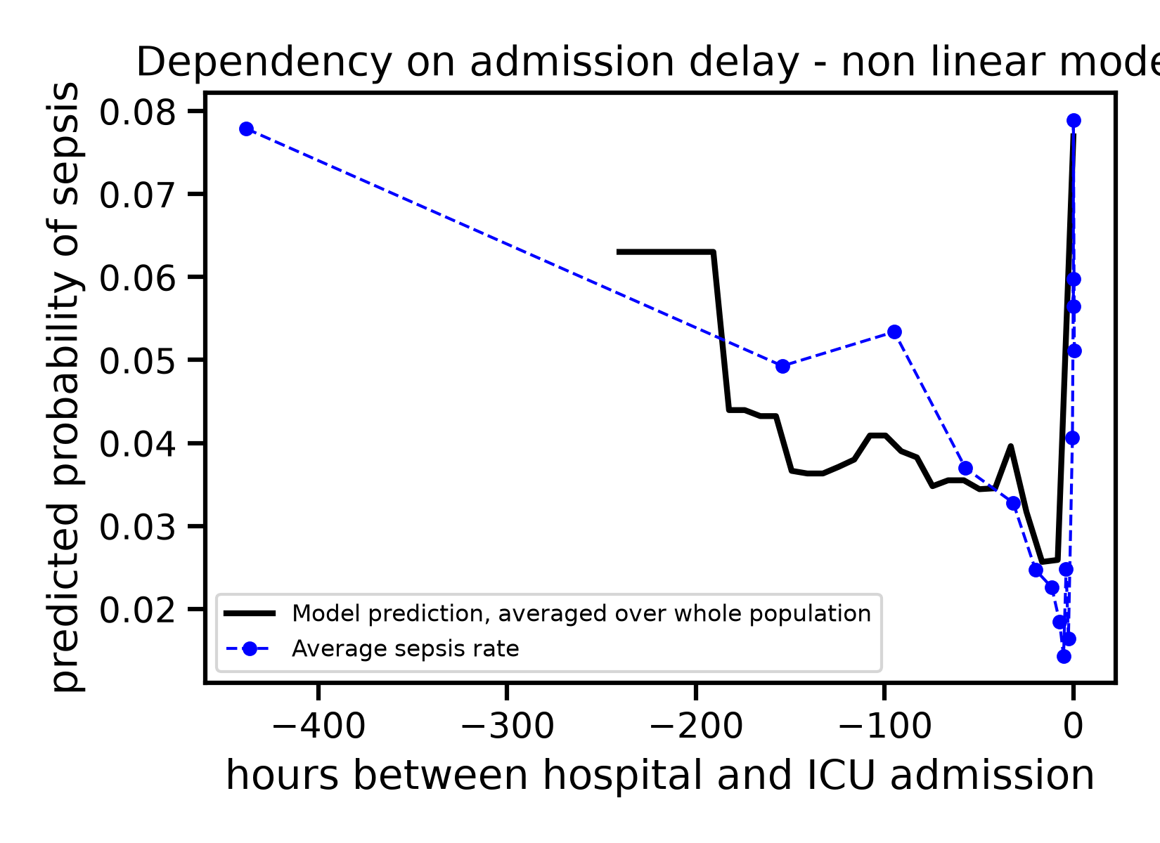
Here we plot “partial dependencies”, that show how the prediction of the model for this feature changes, on average, across the population.

A few patients are missing a diastolic blood pressure reading, so we first drop them: the model can handle missing values internally, but the plotting code below cannot.

X_test_delay = X_test.dropna(subset=["hours_before_icu"])
y_test_delay = y_test.loc[X_test_delay.index]

We will plot local averages of the observed sepsis rate, to compare with the model’s predictions. For this, we need to group patients by delay into 16 bins of equal size before averaging observed sepsis.

observed_delay = X_test_delay[["sex", "hours_before_icu"]].copy()
observed_delay["sepsis"] = y_test_delay
observed_delay["delay_bin"] = pd.qcut(observed_delay["hours_before_icu"], q=16)

For the linear model

import matplotlib.pyplot as plt
from sklearn.inspection import partial_dependence
pd_population_linear_delay = partial_dependence(
    model_linear, X_test_delay, features=["hours_before_icu"], grid_resolution=30
)

plt.figure()
plt.plot(
    pd_population_linear_delay["grid_values"][0],
    pd_population_linear_delay["average"][0],
    color="black",
    linewidth=2,
    label="Model prediction, averaged over whole population",
)

observed_by_bin = observed_delay.groupby("delay_bin")[["hours_before_icu", "sepsis"]].mean()
plt.plot(
    observed_by_bin["hours_before_icu"],
    observed_by_bin["sepsis"],
    color='blue',
    linewidth=1,
    linestyle="--",
    marker='o',
    markersize=4,
    label="Average sepsis rate",
)

plt.xlabel("hours between hospital and ICU admission")
plt.ylabel("predicted probability of sepsis")
plt.title("Dependency on admission delay - linear model")
plt.legend(fontsize=8)
plt.tight_layout()
plt.show()

/home/runner/work/health_ml_tutorial/health_ml_tutorial/examples/01_predict_icu_sepsis.py:190: FutureWarning: The default of observed=False is deprecated and will be changed to True in a future version of pandas. Pass observed=False to retain current behavior or observed=True to adopt the future default and silence this warning.
  observed_by_bin = observed_delay.groupby("delay_bin")[["hours_before_icu", "sepsis"]].mean()

The non-linear model instead traces a bumpy, non-monotonic curve. It is likely that these bumps reflect noise in addition to real link between admission delay and sepsis, but this model predicts better the observed sepsis rate than the linear model: the actual dynamics are likely not monotonic.

For the non-linear model

pd_population_nonlinear_delay = partial_dependence(
    model_nonlinear, X_test_delay, features=["hours_before_icu"], grid_resolution=30
)

plt.figure()
plt.plot(
    pd_population_nonlinear_delay["grid_values"][0],
    pd_population_nonlinear_delay["average"][0],
    color="black",
    linewidth=2,
    label="Model prediction, averaged over whole population",
)

observed_by_bin = observed_delay.groupby("delay_bin")[["hours_before_icu", "sepsis"]].mean()
plt.plot(
    observed_by_bin["hours_before_icu"],
    observed_by_bin["sepsis"],
    color='blue',
    linewidth=1,
    linestyle="--",
    marker='o',
    markersize=4,
    label="Average sepsis rate",
)


plt.xlabel("hours between hospital and ICU admission")
plt.ylabel("predicted probability of sepsis")
plt.title("Dependency on admission delay - non linear model")
plt.legend(fontsize=8)
plt.tight_layout()
plt.show()

/home/runner/work/health_ml_tutorial/health_ml_tutorial/examples/01_predict_icu_sepsis.py:233: FutureWarning: The default of observed=False is deprecated and will be changed to True in a future version of pandas. Pass observed=False to retain current behavior or observed=True to adopt the future default and silence this warning.
  observed_by_bin = observed_delay.groupby("delay_bin")[["hours_before_icu", "sepsis"]].mean()