
Note
Go to the end to download the full example code or to run this example in your browser via JupyterLite or Binder.
Trade-offs in model flexibility#
More flexible models are not always better: they need a lot of data (100k individuals is small by machine-learning standards, though much large than typical health dataset). The risk of using too flexible a model is to capture noise.
Using the same PhysioNet sepsis data as the previous example, we push a single, easy-to-reason-about “flexibility” knob - the maximum depth of a decision tree - hard in both directions, to see under-fitting and over-fitting happen concretely. We then look at why averaging many trees (a random forest) tames over-fitting, and how more data pushes the same model from over-fitting to a good fit.
Learning objectives and take home messages#
This notebook shows how the most flexible model is not always the best.
It can be skipped if you’re in a hurry.
Load the data and split train / test#
import pandas as pd
df = pd.read_csv("physionet_sepsis.csv")
Quick display of the data
from skrub import TableReport
TableReport(df)
| age | sex | hours_before_icu | diastolic_bp_mmhg | sepsis | |
|---|---|---|---|---|---|
| 0 | 83.1 | F | -0.0300 | 0 | |
| 1 | 75.9 | F | -98.6 | 44.1 | 0 |
| 2 | 45.8 | F | -1.20e+03 | 52.2 | 0 |
| 3 | 65.7 | F | -8.77 | 51.4 | 0 |
| 4 | 28.1 | M | -0.0500 | 0 | |
| 38,962 | 84.0 | F | -6.69 | 74.6 | 0 |
| 38,963 | 30.0 | M | -0.0200 | 70.3 | 0 |
| 38,964 | 60.0 | F | -53.6 | 83.1 | 0 |
| 38,965 | 84.0 | F | -10.7 | 74.4 | 0 |
| 38,966 | 62.0 | F | 0.00 | 72.7 | 0 |
age
Float64DType- Null values
- 15 (< 0.1%)
- Unique values
-
9,162 (23.5%)
This column has a high cardinality (> 40).
- Mean ± Std
- 61.6 ± 16.5
- Median ± IQR
- 63.2 ± 23.0
- Min | Max
- 14.0 | 100.
sex
ObjectDType- Null values
- 0 (0.0%)
- Unique values
- 2 (< 0.1%)
Most frequent values
hours_before_icu
Float64DType- Null values
- 1 (< 0.1%)
- Unique values
-
11,845 (30.4%)
This column has a high cardinality (> 40).
- Mean ± Std
- -50.7 ± 136.
- Median ± IQR
- -6.13 ± 43.1
- Min | Max
- -5.37e+03 | 24.0
diastolic_bp_mmhg
Float64DType- Null values
- 7,512 (19.3%)
- Unique values
-
11,293 (29.0%)
This column has a high cardinality (> 40).
- Mean ± Std
- 64.1 ± 11.2
- Median ± IQR
- 62.8 ± 14.5
- Min | Max
- 25.0 | 149.
sepsis
Int64DType- Null values
- 0 (0.0%)
- Unique values
- 2 (< 0.1%)
- Mean ± Std
- 0.0405 ± 0.197
- Median ± IQR
- 0 ± 0
- Min | Max
- 0 | 1
No columns match the selected filter: . You can change the column filter in the dropdown menu above.
| Column | Column name | dtype | Is sorted | Null values | Unique values | Mean | Std | Min | Median | Max |
|---|---|---|---|---|---|---|---|---|---|---|
| 0 | age | Float64DType | False | 15 (< 0.1%) | 9162 (23.5%) | 61.6 | 16.5 | 14.0 | 63.2 | 100. |
| 1 | sex | ObjectDType | False | 0 (0.0%) | 2 (< 0.1%) | |||||
| 2 | hours_before_icu | Float64DType | False | 1 (< 0.1%) | 11845 (30.4%) | -50.7 | 136. | -5.37e+03 | -6.13 | 24.0 |
| 3 | diastolic_bp_mmhg | Float64DType | False | 7512 (19.3%) | 11293 (29.0%) | 64.1 | 11.2 | 25.0 | 62.8 | 149. |
| 4 | sepsis | Int64DType | False | 0 (0.0%) | 2 (< 0.1%) | 0.0405 | 0.197 | 0 | 0 | 1 |
No columns match the selected filter: . You can change the column filter in the dropdown menu above.
age
Float64DType- Null values
- 15 (< 0.1%)
- Unique values
-
9,162 (23.5%)
This column has a high cardinality (> 40).
- Mean ± Std
- 61.6 ± 16.5
- Median ± IQR
- 63.2 ± 23.0
- Min | Max
- 14.0 | 100.
sex
ObjectDType- Null values
- 0 (0.0%)
- Unique values
- 2 (< 0.1%)
Most frequent values
hours_before_icu
Float64DType- Null values
- 1 (< 0.1%)
- Unique values
-
11,845 (30.4%)
This column has a high cardinality (> 40).
- Mean ± Std
- -50.7 ± 136.
- Median ± IQR
- -6.13 ± 43.1
- Min | Max
- -5.37e+03 | 24.0
diastolic_bp_mmhg
Float64DType- Null values
- 7,512 (19.3%)
- Unique values
-
11,293 (29.0%)
This column has a high cardinality (> 40).
- Mean ± Std
- 64.1 ± 11.2
- Median ± IQR
- 62.8 ± 14.5
- Min | Max
- 25.0 | 149.
sepsis
Int64DType- Null values
- 0 (0.0%)
- Unique values
- 2 (< 0.1%)
- Mean ± Std
- 0.0405 ± 0.197
- Median ± IQR
- 0 ± 0
- Min | Max
- 0 | 1
No columns match the selected filter: . You can change the column filter in the dropdown menu above.
| Column 1 | Column 2 | Cramér's V | Pearson's Correlation |
|---|---|---|---|
| age | diastolic_bp_mmhg | 0.137 | -0.352 |
| age | sex | 0.0776 | |
| diastolic_bp_mmhg | sepsis | 0.0674 | -0.0599 |
| hours_before_icu | sepsis | 0.0659 | -0.0466 |
| sex | diastolic_bp_mmhg | 0.0658 | |
| sex | hours_before_icu | 0.0584 | |
| hours_before_icu | diastolic_bp_mmhg | 0.0554 | 0.0963 |
| age | hours_before_icu | 0.0490 | -0.0252 |
| age | sepsis | 0.0411 | 0.0155 |
| sex | sepsis | 0.00545 |
Please enable javascript
The skrub table reports need javascript to display correctly. If you are displaying a report in a Jupyter notebook and you see this message, you may need to re-execute the cell or to trust the notebook (button on the top right or "File > Trust notebook").
Our features, target, and a train-test split
A single decision tree: one knob for flexibility#
A decision tree predicts by asking a sequence of yes/no questions
about the covariates, which end up defining bins for continuous
variables. Its max_depth sets how many questions can be
chained before making a prediction: a shallow tree can only represent
a simple, rigid rule, while a deep tree can carve out a rule specific
to almost every individual patient in the training set.
We fit one tree per depth, and score it both on the data it was trained on and on the held-out test set.
from sklearn.metrics import roc_auc_score
from sklearn.tree import DecisionTreeClassifier
from skrub import tabular_pipeline

max_depths = [1, 2, 3, 4, 5, 6, 8, 10, 12, 15, 20, None]

train_scores, test_scores = [], []
for max_depth in max_depths:
    model = tabular_pipeline(DecisionTreeClassifier(max_depth=max_depth, random_state=0))
    model.fit(X_train, y_train)
    train_scores.append(roc_auc_score(y_train, model.predict_proba(X_train)[:, 1]))
    test_scores.append(roc_auc_score(y_test, model.predict_proba(X_test)[:, 1]))
    print(f"max_depth={str(max_depth):5s}  train AUC={train_scores[-1]:.3f}  test AUC={test_scores[-1]:.3f}")
max_depth=1      train AUC=0.580  test AUC=0.560
max_depth=2      train AUC=0.632  test AUC=0.613
max_depth=3      train AUC=0.664  test AUC=0.649
max_depth=4      train AUC=0.682  test AUC=0.651
max_depth=5      train AUC=0.692  test AUC=0.649
max_depth=6      train AUC=0.704  test AUC=0.643
max_depth=8      train AUC=0.739  test AUC=0.636
max_depth=10     train AUC=0.781  test AUC=0.623
max_depth=12     train AUC=0.842  test AUC=0.590
max_depth=15     train AUC=0.915  test AUC=0.583
max_depth=20     train AUC=0.983  test AUC=0.547
max_depth=None   train AUC=1.000  test AUC=0.509
Plotting train and test performance side by side makes the two failure modes obvious.
import matplotlib.pyplot as plt

# A plain integer x-axis, with "None" (unlimited depth) placed one step
# after the deepest limited depth.
x_positions = range(len(max_depths))
x_labels = []
for max_depth in max_depths:
    if max_depth is None:
        x_labels.append("None\n(unlimited)")
    else:
        x_labels.append(str(max_depth))

plt.plot(x_positions, train_scores, marker="o", label="Train AUC")
plt.plot(x_positions, test_scores, marker="o", label="Test AUC")
plt.xticks(list(x_positions), x_labels)
plt.xlabel("max_depth (tree flexibility)")
plt.ylabel("AUC")
plt.title("A single decision tree: under-fitting to over-fitting")
plt.legend()
plt.tight_layout()
plt.show()
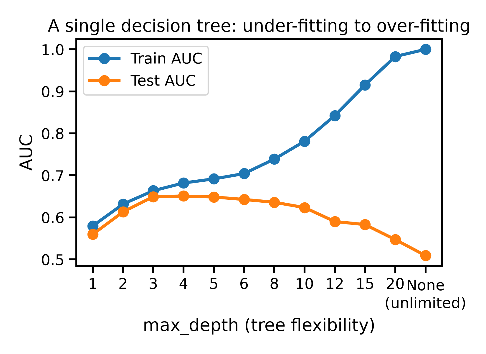
On the left (small max_depth), the tree is too rigid: it cannot
even fit the training data well (train AUC is low), and it does no
better on the test set. This is under-fitting.
On the right (max_depth=None), the tree perfectly memorizes the
training data (train AUC = 1.0), but test performance collapses to
worse than a coin flip. This is over-fitting: the tree has learned the
noise specific to the training patients, not the pattern that
generalizes. With sepsis this rare (~4% of patients), a deep tree can
carve out leaves containing a handful of patients, or even one, and
treat their exact outcome as a hard rule.
In between, around max_depth=4, test performance peaks: the tree
is flexible enough to capture real structure, but not so flexible that
it chases noise. Only the held-out test set lets us find this sweet
spot - the training score alone keeps improving all the way to the
right, and would be a misleading guide on its own.
What the extremes actually look like#
To make “under-fit” and “over-fit” concrete rather than abstract, we look at the partial dependence of the delay before ICU admission - the clearest non-linear feature in the previous example - at three depths: too shallow, the sweet spot, and unlimited.
from sklearn.inspection import partial_dependence

# A few patients are missing this reading, so we first drop them: the
# model can handle missing values internally, but the plotting code
# below cannot.
X_train_complete = X_train.dropna(subset=["hours_before_icu"])
y_train_complete = y_train.loc[X_train_complete.index]

depth_labels = ["under-fit (max_depth=1)", "sweet spot (max_depth=4)", "over-fit (max_depth=None)"]
depth_values = [1, 4, None]

fig, axes = plt.subplots(1, 3, figsize=(15, 4.5), sharey=True)

for i in range(3):
    ax = axes[i]
    label = depth_labels[i]
    max_depth = depth_values[i]

    model = tabular_pipeline(DecisionTreeClassifier(max_depth=max_depth, random_state=0))
    model.fit(X_train_complete, y_train_complete)
    pd_result = partial_dependence(
        model, X_train_complete, features=["hours_before_icu"], grid_resolution=100
    )
    ax.plot(pd_result["grid_values"][0], pd_result["average"][0], color="black")
    ax.set_xlabel("hours before ICU admission")
    ax.set_title(label)

axes[0].set_ylabel("predicted probability of sepsis")
fig.tight_layout()
plt.show()
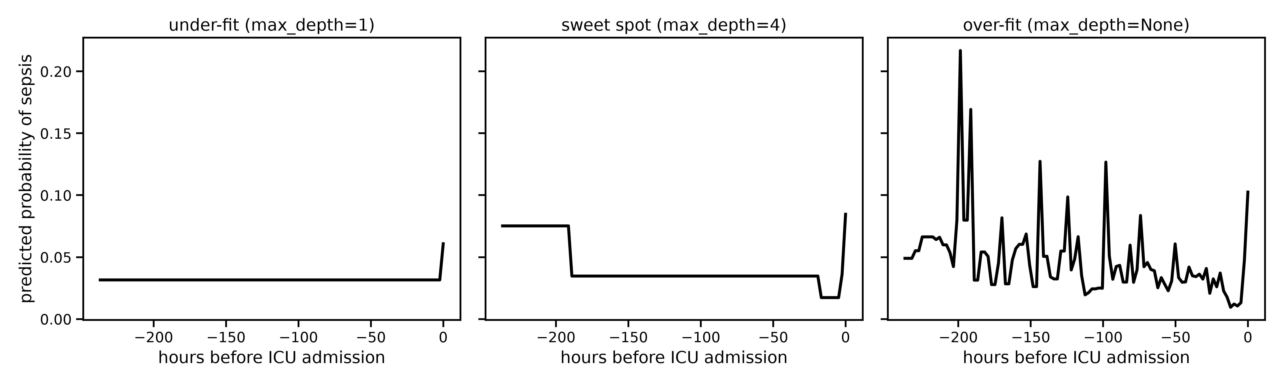
The under-fit tree can only ask one yes/no question, so it collapses the real curve into a single step: patients admitted right away versus everyone else. The sweet-spot tree in the middle traces a much more plausible multi-step curve: risk is elevated for the longest delays, dips for intermediate ones, and rises sharply for immediate admissions. The over-fit tree is a wild, jagged staircase, chasing every idiosyncrasy of the training patients.
Averaging many trees tames over-fitting#
A random forest fits many trees, each on a bootstrap resample of the
data, and averages their predictions. This averaging cancels out a lot
of the noise any single deep tree picks up, without giving up
flexibility. We repeat the same max_depth sweep with a random
forest, and compare its test curve to the single tree’s.
from sklearn.ensemble import RandomForestClassifier

forest_test_scores = []
for max_depth in max_depths:
    model = tabular_pipeline(RandomForestClassifier(max_depth=max_depth, random_state=0))
    model.fit(X_train, y_train)
    forest_test_scores.append(roc_auc_score(y_test, model.predict_proba(X_test)[:, 1]))

plt.figure()
plt.plot(x_positions, test_scores, marker="o", label="Single tree, test AUC")
plt.plot(x_positions, forest_test_scores, marker="o", label="Random forest, test AUC")
plt.xticks(list(x_positions), x_labels)
plt.xlabel("max_depth (tree flexibility)")
plt.ylabel("Test AUC")
plt.title("Averaging many trees is far more robust to over-fitting")
plt.legend()
plt.tight_layout()
plt.show()
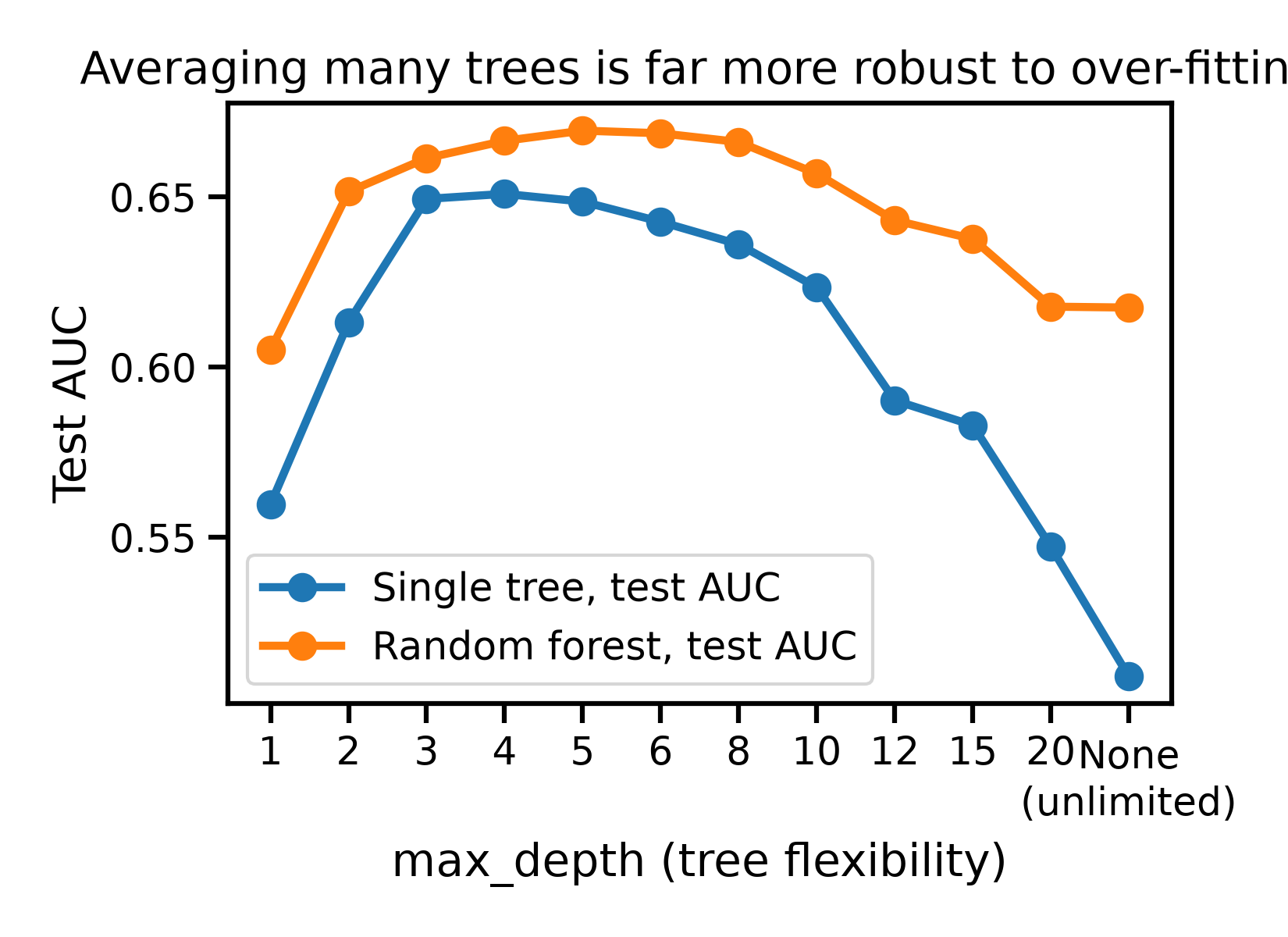
The random forest’s test performance drops much more gently at large
depths than the single tree’s collapse - though on this rare-event
task, it still drops. Unlike the previous ICU-mortality example, here
there is no depth at which a random forest is a safe “set it deep and
forget it” choice: some care in choosing max_depth still pays off.
Asymptotics: more data turns over-fitting into a good fit#
Over-fitting is not just a property of the model: it is a property of
the model relative to how much data we have. We fix a single tree
at max_depth=4 - the sweet spot we found above with the full
training set - and refit it on growing subsets of the training data,
to see what happens with less, or more, data.
sample_sizes = [200, 500, 1000, 2000, 5000, 10000, len(X_train)]

train_scores_by_n, test_scores_by_n = [], []
for n in sample_sizes:
    X_sub = X_train.iloc[:n]
    y_sub = y_train.iloc[:n]
    model = tabular_pipeline(DecisionTreeClassifier(max_depth=4, random_state=0))
    model.fit(X_sub, y_sub)
    train_scores_by_n.append(roc_auc_score(y_sub, model.predict_proba(X_sub)[:, 1]))
    test_scores_by_n.append(roc_auc_score(y_test, model.predict_proba(X_test)[:, 1]))
    print(f"n={n:6d}  train AUC={train_scores_by_n[-1]:.3f}  test AUC={test_scores_by_n[-1]:.3f}")

plt.figure()
plt.plot(sample_sizes, train_scores_by_n, marker="o", label="Train AUC")
plt.plot(sample_sizes, test_scores_by_n, marker="o", label="Test AUC")
plt.xscale("log")
plt.xlabel("Number of training samples")
plt.ylabel("AUC")
plt.title("A depth-4 tree: over-fitting shrinks as training data grows")
plt.legend()
plt.tight_layout()
plt.show()
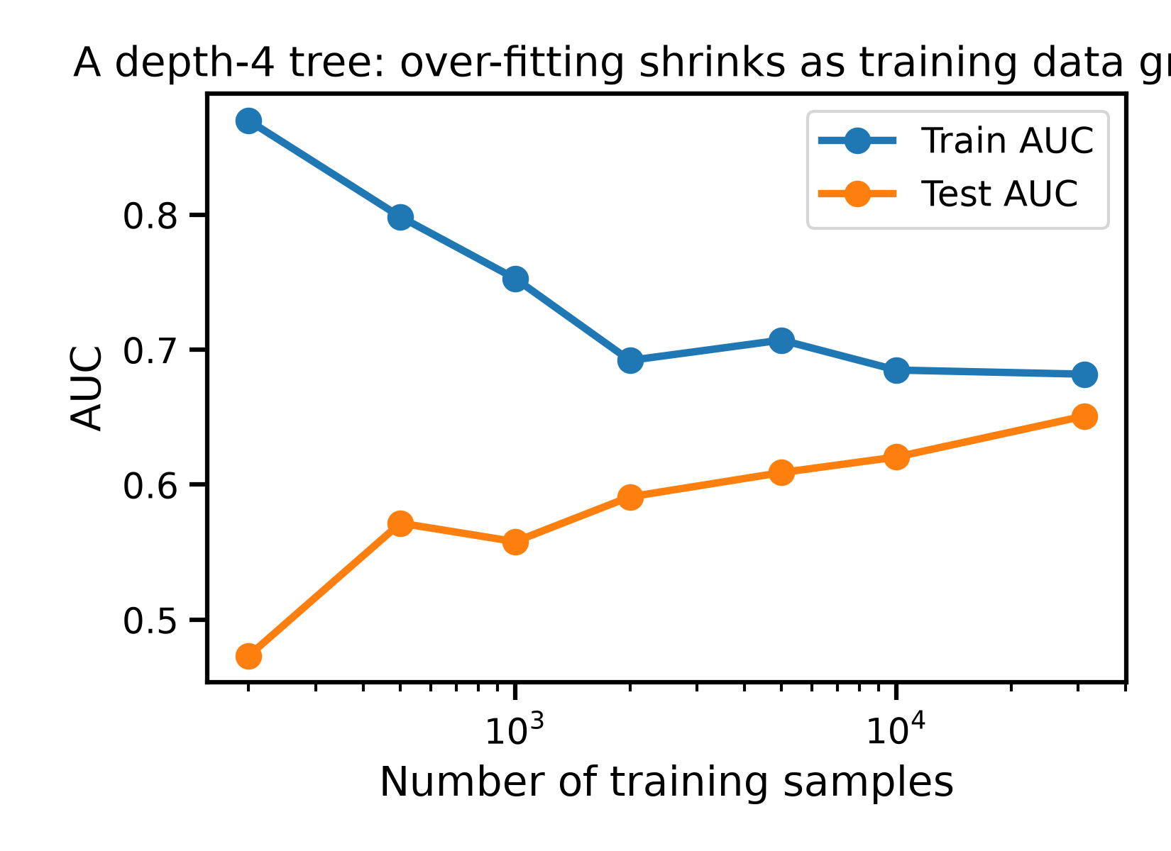
n=   200  train AUC=0.870  test AUC=0.473
n=   500  train AUC=0.798  test AUC=0.572
n=  1000  train AUC=0.753  test AUC=0.558
n=  2000  train AUC=0.692  test AUC=0.591
n=  5000  train AUC=0.707  test AUC=0.609
n= 10000  train AUC=0.685  test AUC=0.620
n= 31173  train AUC=0.682  test AUC=0.651
With only 200 training patients, this same depth-4 tree is actively harmful (test AUC below 0.5, worse than a coin flip): with sepsis this rare, 200 patients contain only a handful of sepsis cases, far too few to estimate reliable probabilities in each leaf of the tree. As the training set grows towards its full size, train and test AUC converge, and test performance keeps improving. The model’s flexibility did not change - only the amount of data did. This is the asymptotic behaviour that makes flexible, non-parametric models useful in the first place: give them enough data, and they can approach the true underlying relationship.
Total running time of the script: (0 minutes 52.206 seconds)

