
Note
Go to the end to download the full example code or to run this example in your browser via JupyterLite or Binder.
Survival and time-to-event: accounting for censoring#
In the NHANES mortality data participant we know months_in_study
(their follow-up duration) and event (whether they died, or were
still alive - “censored” - at the end of follow-up). We can use it in a
time-to-event question, studying the time people live, ie a survival
question.
And yet, there is a challenge: censoring. Participants enrolled towards the end of the study simply have not been followed long enough to know if or when they will die: their true time to death is unknown, only a lower bound on it.
We first show what goes wrong if this censoring is ignored: predicting
“time to death” using only the participants who died. We then show how
a proper survival model - SurvivalBoost from the hazardous library - uses the censored
participants too, without needing to know their exact time of death.
Learning objectives and take home messages#
When following individuals to observe an event (such as death), the observation period may often be too small to observe this event for all individuals. Dropping the individuals for which the event is not observed creates a bias. The right solution is to use techniques known as “survival analysis”.
The data: an epidemiological cohort#
import pandas as pd

df = pd.read_csv("nhanes_1999_2018_mortality.csv")
A quick glance at the data
from skrub import TableReport
TableReport(df)
| participant_id | cycle | age | sex | race_eth | education | bmi | waist_cm | systolic_bp_mmhg | diastolic_bp_mmhg | EVER_SMOKED | months_in_study | event | |
|---|---|---|---|---|---|---|---|---|---|---|---|---|---|
| 0 | 2.00 | 1999-2000 | 77.0 | M | Non-Hispanic White | 5.00 | 24.9 | 98.0 | 101. | 56.7 | no | 177. | deceased |
| 1 | 5.00 | 1999-2000 | 49.0 | M | Non-Hispanic White | 5.00 | 29.1 | 99.9 | 122. | 82.7 | yes | 244. | alive |
| 2 | 6.00 | 1999-2000 | 19.0 | F | Other race - including multi-racial | 22.6 | 81.6 | 115. | 68.0 | 245. | alive | ||
| 3 | 7.00 | 1999-2000 | 59.0 | F | Non-Hispanic Black | 2.00 | 29.4 | 90.7 | 125. | 80.0 | yes | 236. | alive |
| 4 | 10.0 | 1999-2000 | 43.0 | M | Non-Hispanic Black | 3.00 | 30.9 | 108. | 145. | 96.0 | yes | 231. | deceased |
| 56,248 | 1.03e+05 | 2017-2018 | 33.0 | M | Non-Hispanic White | 3.00 | 23.7 | 85.5 | 122. | 76.7 | yes | 34.0 | alive |
| 56,249 | 1.03e+05 | 2017-2018 | 70.0 | F | Other race - including multi-racial | 3.00 | 20.0 | 82.2 | 139. | 73.3 | no | 34.0 | alive |
| 56,250 | 1.03e+05 | 2017-2018 | 42.0 | M | Mexican American | 3.00 | 35.8 | 115. | 121. | 75.3 | yes | 30.0 | alive |
| 56,251 | 1.03e+05 | 2017-2018 | 41.0 | F | Non-Hispanic Black | 5.00 | 26.1 | 86.4 | 116. | 70.7 | no | 17.0 | alive |
| 56,252 | 1.03e+05 | 2017-2018 | 38.0 | M | Non-Hispanic White | 4.00 | 36.1 | 122. | 148. | 96.0 | yes | 26.0 | alive |
participant_id
Float64DType- Null values
- 0 (0.0%)
- Unique values
-
56,253 (100.0%)
This column has a high cardinality (> 40).
- Mean ± Std
- 5.28e+04 ± 2.95e+04
- Median ± IQR
- 5.32e+04 ± 5.12e+04
- Min | Max
- 2.00 | 1.03e+05
cycle
ObjectDType- Null values
- 0 (0.0%)
- Unique values
- 10 (< 0.1%)
Most frequent values
age
Float64DType- Null values
- 0 (0.0%)
- Unique values
-
68 (0.1%)
This column has a high cardinality (> 40).
- Mean ± Std
- 47.5 ± 19.3
- Median ± IQR
- 46.0 ± 32.0
- Min | Max
- 18.0 | 85.0
sex
ObjectDType- Null values
- 0 (0.0%)
- Unique values
- 2 (< 0.1%)
Most frequent values
race_eth
ObjectDType- Null values
- 0 (0.0%)
- Unique values
- 5 (< 0.1%)
Most frequent values
education
Float64DType- Null values
- 3,967 (7.1%)
- Unique values
- 7 (< 0.1%)
- Mean ± Std
- 3.32 ± 1.31
- Median ± IQR
- 3.00 ± 2.00
- Min | Max
- 1.00 | 9.00
bmi
Float64DType- Null values
- 1,155 (2.1%)
- Unique values
-
3,547 (6.3%)
This column has a high cardinality (> 40).
- Mean ± Std
- 28.7 ± 6.84
- Median ± IQR
- 27.6 ± 8.14
- Min | Max
- 12.0 | 130.
waist_cm
Float64DType- Null values
- 3,180 (5.7%)
- Unique values
-
1,030 (1.8%)
This column has a high cardinality (> 40).
- Mean ± Std
- 97.8 ± 16.3
- Median ± IQR
- 96.7 ± 21.6
- Min | Max
- 55.5 | 179.
systolic_bp_mmhg
Float64DType- Null values
- 2,591 (4.6%)
- Unique values
-
313 (0.6%)
This column has a high cardinality (> 40).
- Mean ± Std
- 124. ± 19.5
- Median ± IQR
- 121. ± 23.3
- Min | Max
- 64.7 | 270.
diastolic_bp_mmhg
Float64DType- Null values
- 2,591 (4.6%)
- Unique values
-
240 (0.4%)
This column has a high cardinality (> 40).
- Mean ± Std
- 69.6 ± 13.4
- Median ± IQR
- 70.0 ± 15.3
- Min | Max
- 5.40e-79 | 139.
EVER_SMOKED
ObjectDType- Null values
- 3,108 (5.5%)
- Unique values
- 4 (< 0.1%)
Most frequent values
months_in_study
Float64DType- Null values
- 0 (0.0%)
- Unique values
-
250 (0.4%)
This column has a high cardinality (> 40).
- Mean ± Std
- 117. ± 67.2
- Median ± IQR
- 113. ± 111.
- Min | Max
- 0.00 | 249.
event
ObjectDType- Null values
- 0 (0.0%)
- Unique values
- 2 (< 0.1%)
Most frequent values
No columns match the selected filter: . You can change the column filter in the dropdown menu above.
| Column | Column name | dtype | Is sorted | Null values | Unique values | Mean | Std | Min | Median | Max |
|---|---|---|---|---|---|---|---|---|---|---|
| 0 | participant_id | Float64DType | True | 0 (0.0%) | 56253 (100.0%) | 5.28e+04 | 2.95e+04 | 2.00 | 5.32e+04 | 1.03e+05 |
| 1 | cycle | ObjectDType | True | 0 (0.0%) | 10 (< 0.1%) | |||||
| 2 | age | Float64DType | False | 0 (0.0%) | 68 (0.1%) | 47.5 | 19.3 | 18.0 | 46.0 | 85.0 |
| 3 | sex | ObjectDType | False | 0 (0.0%) | 2 (< 0.1%) | |||||
| 4 | race_eth | ObjectDType | False | 0 (0.0%) | 5 (< 0.1%) | |||||
| 5 | education | Float64DType | False | 3967 (7.1%) | 7 (< 0.1%) | 3.32 | 1.31 | 1.00 | 3.00 | 9.00 |
| 6 | bmi | Float64DType | False | 1155 (2.1%) | 3547 (6.3%) | 28.7 | 6.84 | 12.0 | 27.6 | 130. |
| 7 | waist_cm | Float64DType | False | 3180 (5.7%) | 1030 (1.8%) | 97.8 | 16.3 | 55.5 | 96.7 | 179. |
| 8 | systolic_bp_mmhg | Float64DType | False | 2591 (4.6%) | 313 (0.6%) | 124. | 19.5 | 64.7 | 121. | 270. |
| 9 | diastolic_bp_mmhg | Float64DType | False | 2591 (4.6%) | 240 (0.4%) | 69.6 | 13.4 | 5.40e-79 | 70.0 | 139. |
| 10 | EVER_SMOKED | ObjectDType | False | 3108 (5.5%) | 4 (< 0.1%) | |||||
| 11 | months_in_study | Float64DType | False | 0 (0.0%) | 250 (0.4%) | 117. | 67.2 | 0.00 | 113. | 249. |
| 12 | event | ObjectDType | False | 0 (0.0%) | 2 (< 0.1%) |
No columns match the selected filter: . You can change the column filter in the dropdown menu above.
participant_id
Float64DType- Null values
- 0 (0.0%)
- Unique values
-
56,253 (100.0%)
This column has a high cardinality (> 40).
- Mean ± Std
- 5.28e+04 ± 2.95e+04
- Median ± IQR
- 5.32e+04 ± 5.12e+04
- Min | Max
- 2.00 | 1.03e+05
cycle
ObjectDType- Null values
- 0 (0.0%)
- Unique values
- 10 (< 0.1%)
Most frequent values
age
Float64DType- Null values
- 0 (0.0%)
- Unique values
-
68 (0.1%)
This column has a high cardinality (> 40).
- Mean ± Std
- 47.5 ± 19.3
- Median ± IQR
- 46.0 ± 32.0
- Min | Max
- 18.0 | 85.0
sex
ObjectDType- Null values
- 0 (0.0%)
- Unique values
- 2 (< 0.1%)
Most frequent values
race_eth
ObjectDType- Null values
- 0 (0.0%)
- Unique values
- 5 (< 0.1%)
Most frequent values
education
Float64DType- Null values
- 3,967 (7.1%)
- Unique values
- 7 (< 0.1%)
- Mean ± Std
- 3.32 ± 1.31
- Median ± IQR
- 3.00 ± 2.00
- Min | Max
- 1.00 | 9.00
bmi
Float64DType- Null values
- 1,155 (2.1%)
- Unique values
-
3,547 (6.3%)
This column has a high cardinality (> 40).
- Mean ± Std
- 28.7 ± 6.84
- Median ± IQR
- 27.6 ± 8.14
- Min | Max
- 12.0 | 130.
waist_cm
Float64DType- Null values
- 3,180 (5.7%)
- Unique values
-
1,030 (1.8%)
This column has a high cardinality (> 40).
- Mean ± Std
- 97.8 ± 16.3
- Median ± IQR
- 96.7 ± 21.6
- Min | Max
- 55.5 | 179.
systolic_bp_mmhg
Float64DType- Null values
- 2,591 (4.6%)
- Unique values
-
313 (0.6%)
This column has a high cardinality (> 40).
- Mean ± Std
- 124. ± 19.5
- Median ± IQR
- 121. ± 23.3
- Min | Max
- 64.7 | 270.
diastolic_bp_mmhg
Float64DType- Null values
- 2,591 (4.6%)
- Unique values
-
240 (0.4%)
This column has a high cardinality (> 40).
- Mean ± Std
- 69.6 ± 13.4
- Median ± IQR
- 70.0 ± 15.3
- Min | Max
- 5.40e-79 | 139.
EVER_SMOKED
ObjectDType- Null values
- 3,108 (5.5%)
- Unique values
- 4 (< 0.1%)
Most frequent values
months_in_study
Float64DType- Null values
- 0 (0.0%)
- Unique values
-
250 (0.4%)
This column has a high cardinality (> 40).
- Mean ± Std
- 117. ± 67.2
- Median ± IQR
- 113. ± 111.
- Min | Max
- 0.00 | 249.
event
ObjectDType- Null values
- 0 (0.0%)
- Unique values
- 2 (< 0.1%)
Most frequent values
No columns match the selected filter: . You can change the column filter in the dropdown menu above.
| Column 1 | Column 2 | Cramér's V | Pearson's Correlation |
|---|---|---|---|
| participant_id | cycle | 0.802 | |
| cycle | months_in_study | 0.713 | |
| education | EVER_SMOKED | 0.689 | |
| participant_id | months_in_study | 0.586 | -0.838 |
| bmi | waist_cm | 0.554 | 0.899 |
| age | event | 0.513 | |
| systolic_bp_mmhg | diastolic_bp_mmhg | 0.453 | 0.284 |
| systolic_bp_mmhg | event | 0.290 | |
| age | EVER_SMOKED | 0.276 | |
| participant_id | event | 0.258 | |
| cycle | event | 0.257 | |
| age | education | 0.240 | -0.134 |
| sex | EVER_SMOKED | 0.225 | |
| age | systolic_bp_mmhg | 0.202 | 0.501 |
| education | event | 0.199 | |
| race_eth | education | 0.197 | |
| months_in_study | event | 0.185 | |
| EVER_SMOKED | event | 0.170 | |
| bmi | event | 0.162 | |
| race_eth | event | 0.160 | |
| waist_cm | systolic_bp_mmhg | 0.156 | 0.213 |
| diastolic_bp_mmhg | event | 0.152 | |
| waist_cm | event | 0.150 | |
| age | diastolic_bp_mmhg | 0.149 | -0.0136 |
| sex | bmi | 0.144 | |
| cycle | race_eth | 0.144 | |
| sex | systolic_bp_mmhg | 0.143 | |
| age | waist_cm | 0.143 | 0.260 |
| waist_cm | diastolic_bp_mmhg | 0.133 | 0.109 |
| sex | diastolic_bp_mmhg | 0.130 | |
| participant_id | race_eth | 0.127 | |
| bmi | systolic_bp_mmhg | 0.125 | 0.125 |
| sex | waist_cm | 0.121 | |
| race_eth | months_in_study | 0.118 | |
| EVER_SMOKED | months_in_study | 0.118 | |
| age | race_eth | 0.113 | |
| age | bmi | 0.110 | 0.0855 |
| education | systolic_bp_mmhg | 0.106 | -0.137 |
| age | months_in_study | 0.106 | -0.246 |
| systolic_bp_mmhg | EVER_SMOKED | 0.104 | |
| cycle | EVER_SMOKED | 0.102 | |
| waist_cm | EVER_SMOKED | 0.102 | |
| education | waist_cm | 0.101 | -0.0572 |
| participant_id | EVER_SMOKED | 0.100 | |
| diastolic_bp_mmhg | EVER_SMOKED | 0.0969 | |
| education | diastolic_bp_mmhg | 0.0953 | 0.0858 |
| race_eth | EVER_SMOKED | 0.0856 | |
| race_eth | bmi | 0.0841 | |
| race_eth | diastolic_bp_mmhg | 0.0840 | |
| bmi | EVER_SMOKED | 0.0823 | |
| sex | education | 0.0819 | |
| bmi | diastolic_bp_mmhg | 0.0813 | 0.106 |
| education | bmi | 0.0808 | -0.0539 |
| race_eth | waist_cm | 0.0795 | |
| participant_id | education | 0.0793 | 0.123 |
| cycle | education | 0.0782 | |
| systolic_bp_mmhg | months_in_study | 0.0769 | -0.137 |
| race_eth | systolic_bp_mmhg | 0.0763 | |
| waist_cm | months_in_study | 0.0733 | -0.116 |
| cycle | bmi | 0.0729 | |
| cycle | waist_cm | 0.0707 | |
| education | months_in_study | 0.0707 | -0.0449 |
| cycle | systolic_bp_mmhg | 0.0690 | |
| participant_id | diastolic_bp_mmhg | 0.0689 | 0.0493 |
| participant_id | systolic_bp_mmhg | 0.0684 | -0.0162 |
| cycle | diastolic_bp_mmhg | 0.0683 | |
| participant_id | waist_cm | 0.0662 | 0.0896 |
| cycle | age | 0.0653 | |
| participant_id | bmi | 0.0643 | 0.0822 |
| participant_id | age | 0.0634 | 0.0310 |
| diastolic_bp_mmhg | months_in_study | 0.0614 | 0.00586 |
| bmi | months_in_study | 0.0576 | -0.0644 |
| sex | months_in_study | 0.0531 | |
| age | sex | 0.0497 | |
| sex | race_eth | 0.0485 | |
| sex | event | 0.0470 | |
| participant_id | sex | 0.0457 | |
| cycle | sex | 0.0426 |
Please enable javascript
The skrub table reports need javascript to display correctly. If you are displaying a report in a Jupyter notebook and you see this message, you may need to re-execute the cell or to trust the notebook (button on the top right or "File > Trust notebook").
Our covariates and target
X = df.drop(columns=["participant_id", "cycle", "months_in_study", "event"])
duration = df["months_in_study"]
is_dead = df["event"] == "deceased"

print("Number of participants:", len(df))
print("Deaths observed:", is_dead.sum())
print("Still alive at the end of follow-up (censored):", (~is_dead).sum())
Number of participants: 56253
Deaths observed: 8366
Still alive at the end of follow-up (censored): 47887
The wrong way: dropping the censored participants#
A tempting shortcut is to only keep the participants who died, and fit an ordinary regression model to predict how many months they survived from their covariates. Participants still alive at the end of follow-up are dropped, since we do not know their exact time of death.
from sklearn.model_selection import train_test_split
from skrub import tabular_pipeline

X_dead = X[is_dead]
duration_dead = duration[is_dead]

X_dead_train, X_dead_test, duration_dead_train, duration_dead_test = train_test_split(
    X_dead, duration_dead, test_size=0.2, random_state=0
)

naive_model = tabular_pipeline("regressor")
naive_model.fit(X_dead_train, duration_dead_train)
Evaluated the usual way, on a held-out set of participants who also died, this model looks reasonable.
from sklearn.metrics import mean_absolute_error, r2_score

predicted_dead_test = naive_model.predict(X_dead_test)
print(f"MAE on held-out deaths: {mean_absolute_error(duration_dead_test, predicted_dead_test):.1f} months")
print(f"R2 on held-out deaths: {r2_score(duration_dead_test, predicted_dead_test):.3f}")
MAE on held-out deaths: 45.1 months
R2 on held-out deaths: 0.089
Why it is biased#
Now apply this same model to the participants it never saw: the ones
who were still alive at the end of follow-up. For them, we do not
know their true time to death, but we do know a lower bound on it:
they survived at least months_in_study, since that is how long
they were observed to still be alive.
If the model’s predicted time to death is less than that lower bound, the prediction is not just inaccurate - it is logically impossible: the model predicts these participants should already be dead, when we know for a fact they were not.
X_censored = X[~is_dead]
already_survived = duration[~is_dead]
predicted_censored = naive_model.predict(X_censored)

impossible = predicted_censored < already_survived.values
print(f"Fraction of censored participants with an impossible prediction: {impossible.mean():.1%}")
print(f"Mean predicted time to death (censored): {predicted_censored.mean():.1f} months")
print(f"Mean months already survived (censored): {already_survived.mean():.1f} months")
Fraction of censored participants with an impossible prediction: 58.5%
Mean predicted time to death (censored): 102.8 months
Mean months already survived (censored): 122.8 months
Almost 6 out of 10 censored participants get an impossible prediction. The figure below makes the mechanism clear: predicted time to death is squeezed into a narrow range around the middle of the follow-up window, while participants have already survived up to the full length of the study.
import matplotlib.pyplot as plt

plt.figure()
plt.hist(predicted_censored, bins=50, density=True, alpha=0.6,
         label="predicted time to death")
plt.hist(already_survived, bins=50, density=True, alpha=0.6,
         label="months already survived\n(known lower bound)")
plt.xlabel("months")
plt.ylabel("density")
plt.title("A model trained on deaths only, applied to censored participants")
plt.legend()
plt.tight_layout()
plt.show()
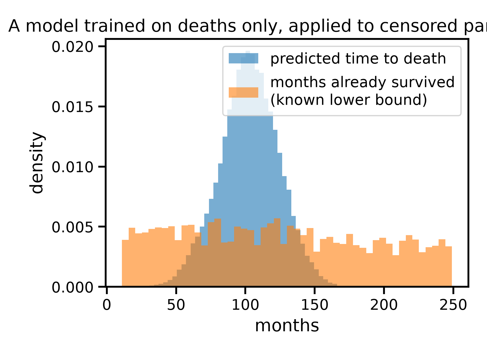
This is not a fluke of this particular model: it follows directly from dropping the censored participants. Among people who died during the study, none of them could have been the healthiest, longest-lived participants - those are exactly the ones still alive, and excluded. The model only ever learns from a population selected for dying within the follow-up window, so it has no way to predict a survival time longer than that window, no matter who it is asked about.
Survival analysis: accounting for censoring properly#
A survival model uses all participants, including the censored
ones, by working with two pieces of information for each of them:
whether the event happened (event), and for how long they were
observed (duration) - censored or not.
A ‘y’ target that exposes censoring#
We build ‘y’ vector that is specific to censoring models, exposing both the duration and if the event we’re interesting (death, here) is observed or not after this duration.
y = pd.DataFrame({
    "event": is_dead.astype(int),
    "duration": duration,
})
This two-column y is exactly the format SurvivalBoost (used
below) expects: a dataframe with columns named "event" and
"duration", "event" being 0 for a censored participant and a
positive integer for an observed event. Passing y this way, instead
of duration alone, is precisely what tells the model which
participants are censored - it never sees an exact time of death for
them, only that they were still alive at their recorded duration.
duration itself plays a double role depending on event: for a
death, it is the exact time to death; for a censored participant, it is
only a lower bound on their (unknown) true time to death - the model
has to treat these two cases differently, and event is what lets
it tell them apart.
The Kaplan-Meier estimator#
Before fitting any model, the Kaplan-Meier estimator gives a
non-parametric estimate of the population’s survival curve - the
probability of still being alive at each point in time - using both
the deaths and the censored participants. Rather than implementing
this ourselves, we use scipy.stats, which has built-in support for
right-censored data through CensoredData: we give it the exact
durations for participants who died (uncensored) and the observed
durations for participants still alive at the end of follow-up
(right, for “right-censored”), and ecdf returns the
Kaplan-Meier survival curve as its survival function .sf.
from scipy.stats import CensoredData, ecdf


def kaplan_meier(duration_values, event_values):
    observed_duration = duration_values[event_values == 1]
    censored_duration = duration_values[event_values == 0]
    survival_function = ecdf(
        CensoredData(uncensored=observed_duration, right=censored_duration)
    ).sf
    time_points = [0] + list(survival_function.quantiles)
    survival_curve = [1.0] + list(survival_function.probabilities)
    return time_points, survival_curve


plt.figure()
time_points, survival_curve = kaplan_meier(y_train["duration"], y_train["event"])
plt.step(time_points, survival_curve, where="post", color="black", label="Whole population")

sex_colors = {"M": "tab:blue", "F": "tab:orange"}
for sex_value, color in sex_colors.items():
    is_sex = X_train["sex"] == sex_value
    time_points_sex, survival_curve_sex = kaplan_meier(
        y_train.loc[is_sex, "duration"], y_train.loc[is_sex, "event"]
    )
    plt.step(time_points_sex, survival_curve_sex, where="post", color=color,
             label=f"sex = {sex_value}")

plt.xlabel("Months")
plt.ylabel("Survival probability")
plt.title("Kaplan-Meier survival curves (training set)")
plt.legend()
plt.tight_layout()
plt.show()
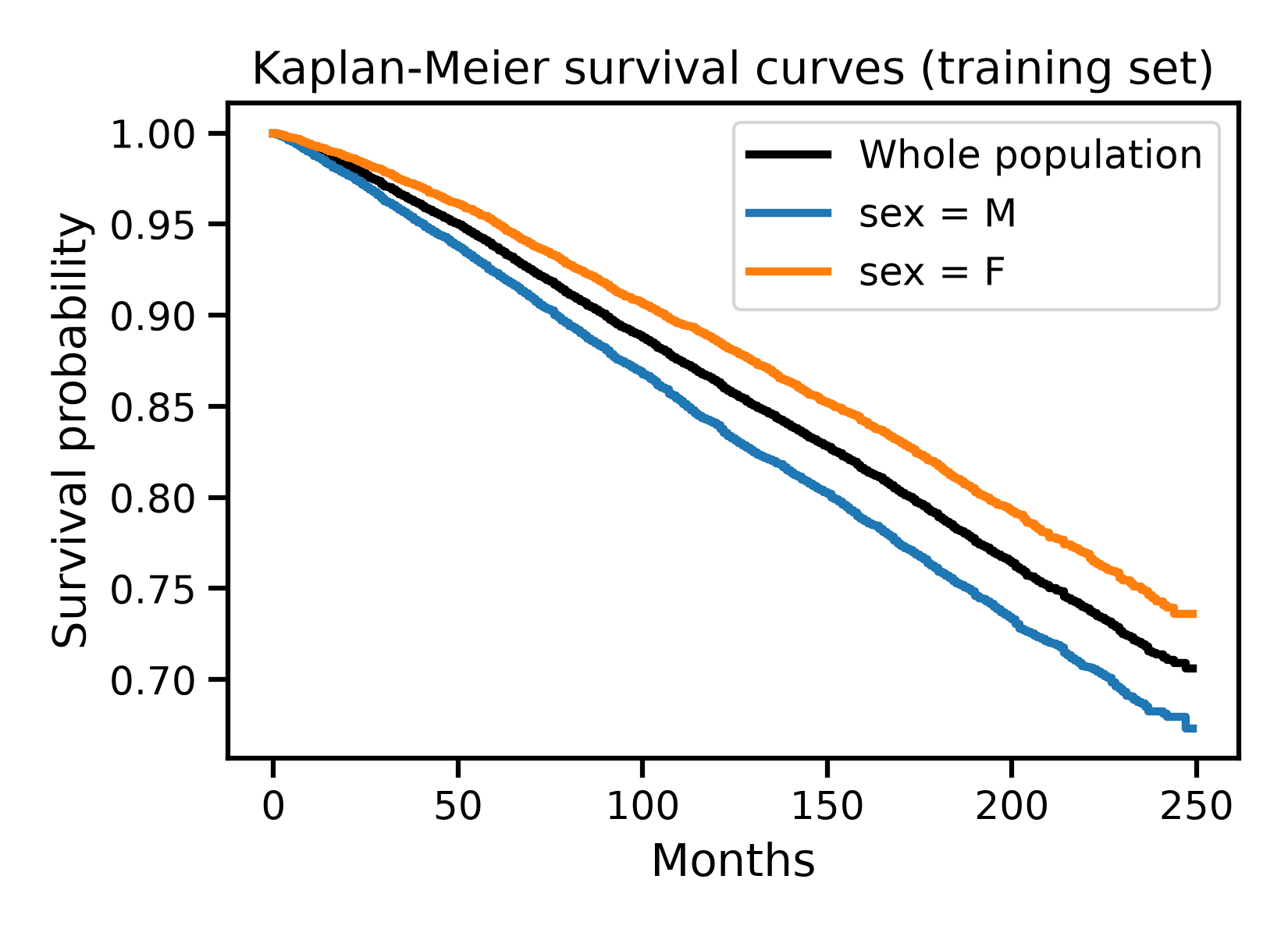
Women have a consistently higher survival probability than men throughout the follow-up period - a well known epidemiological pattern, and a good sanity check that the estimator behaves sensibly.
Fitting SurvivalBoost#
SurvivalBoost is a gradient-boosted survival model: rather than
predicting a single number, it predicts a whole survival curve for
each participant, using every participant - censored or not - during
training. It is described in Alberge, Maladiere, Grisel, Abécassis
and Varoquaux (2025), “Survival Models: Proper Scoring Rule and
Stochastic Optimization with Competing Risks”, Proceedings
of the 28th International Conference on Artificial Intelligence and
Statistics (AISTATS), PMLR 258:3619-3627.
from hazardous import SurvivalBoost

survival_model = tabular_pipeline(
    SurvivalBoost(n_iter=50, show_progressbar=False, random_state=0)
)
survival_model.fit(X_train, y_train)
Predicted survival curves: younger vs older participants#
We compare the predicted survival curves of the 15 youngest and 15 oldest participants in the test set.
survival_boost_model = survival_model.named_steps["survivalboost"]
times = survival_boost_model.time_grid_

X_test_transformed = survival_model[:-1].transform(X_test)
predicted_survival_test = survival_boost_model.predict_survival_function(X_test_transformed)

age_order = X_test["age"].values.argsort()
youngest_index = age_order[:15]
oldest_index = age_order[-15:]

fig, axes = plt.subplots(1, 2, figsize=(11, 4.5), sharey=True)

for index in youngest_index:
    axes[0].plot(times, predicted_survival_test[index], color="tab:blue", alpha=0.5)
for index in oldest_index:
    axes[1].plot(times, predicted_survival_test[index], color="tab:red", alpha=0.5)

axes[0].set_title("15 youngest participants")
axes[1].set_title("15 oldest participants")
for ax in axes:
    ax.set_xlabel("Months")
axes[0].set_ylabel("Predicted survival probability")
fig.tight_layout()
plt.show()
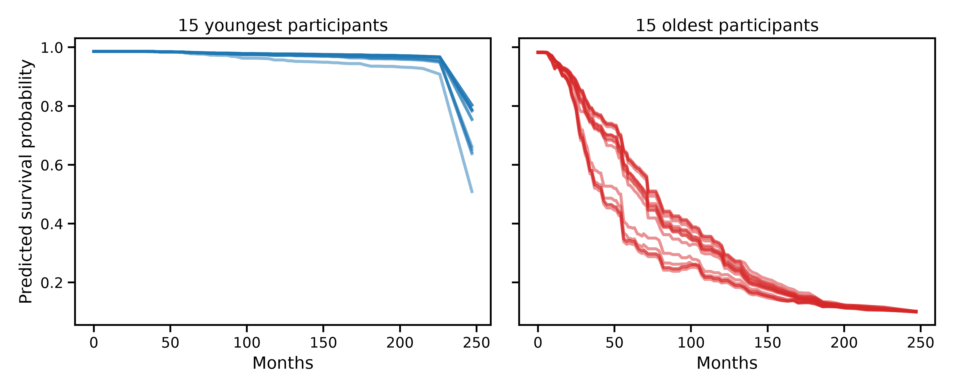
The youngest participants’ predicted survival stays close to 1 throughout follow-up, while the oldest participants’ predicted survival declines much faster and more steeply - exactly the pattern we would expect, and something the naive regression from the first section has no way to express at all.
Calibration: does the predicted risk match what actually happens?#
The integrated Brier score summarizes, across the whole follow-up period, how far predicted survival probabilities are from the actual outcomes - lower is better.
from hazardous.metrics import integrated_brier_score_survival

ibs = integrated_brier_score_survival(y_train, y_test, predicted_survival_test, times)
print(f"Integrated Brier score (test set): {ibs:.3f}")
Integrated Brier score (test set): 0.065
No impossible predictions#
Finally, we repeat the same check as in the first section: for each
censored participant, does the model at least acknowledge they were
alive at the time we know they were? We read, for every test
participant, the predicted survival probability at their own
duration - the exact time of death for those who died, or the
last known “still alive” time for those censored.
import numpy as np

survival_probability_at_own_time = np.zeros(len(X_test))
for i in range(len(X_test)):
    survival_probability_at_own_time[i] = np.interp(
        y_test["duration"].values[i], times, predicted_survival_test[i]
    )

is_censored_test = y_test["event"].values == 0
print(
    "Mean predicted survival probability at participants' own censoring time "
    f"(censored): {survival_probability_at_own_time[is_censored_test].mean():.3f}"
)
print(
    "Mean predicted survival probability at participants' own time of death "
    f"(deaths): {survival_probability_at_own_time[~is_censored_test].mean():.3f}"
)
Mean predicted survival probability at participants' own censoring time (censored): 0.888
Mean predicted survival probability at participants' own time of death (deaths): 0.745
Censored participants get a mean predicted survival probability of about 0.9 at the exact time we know they were still alive - close to certainty, and correctly so. Participants who died get a substantially lower predicted survival probability at their own time of death. Unlike the naive regression, the survival model never contradicts what we already know about a participant’s outcome - it simply has no mechanism to, since it was built from the start to represent that some participants’ true time to event is only known to be “later than this”.
Another approach: finite horizon#
Another way to avoid biases with such righ-censored data is to do a finite-horizon analysis: rather than computing the time that it takes for a given individual to die, choose a time horizon (eg 5 years), keep only individuals that have been observed more than this time, and classify whether after 5 years they were alive or not. This is what we did in the first notebook introducing this dataset. The first drawback of this approach is that it does not give an estimated time, but rather a yes/no answer after a given horizon. One can then use multiple horizons but, by treating each horizon separately, such an approach is less powerful statistically to capture the link between the covariates and the outcome: giving personnalized time-to-events for a given X. It is particularly inefficient at long time horizons, where the censoring depletes massively the cohort. A survival analysis model can learn the link between covariates X and survival for small time horizons where there are many non censored observations, and extrapolate it to large time horizons.
Total running time of the script: (1 minutes 45.912 seconds)

